4.0 - MANAGING RISK & OPPORTUNITY
04.1 - Module 04-1 - Introduction to Managing Risk & Opportunity
04.2 - Module 04-2 - Develop Risk & Opportunity Policies & Procedures Manual
04.3 - Module 04-3 - Identify Risks / Opportunities
04.4 - Module 04-4 - Assess, Prioritize and Quantify Risks / Opportunities
04.5 RISK / OPPORTUNITY RESPONSE STRATEGIES AND TACTICS
04.5.1 - INTRODUCTION
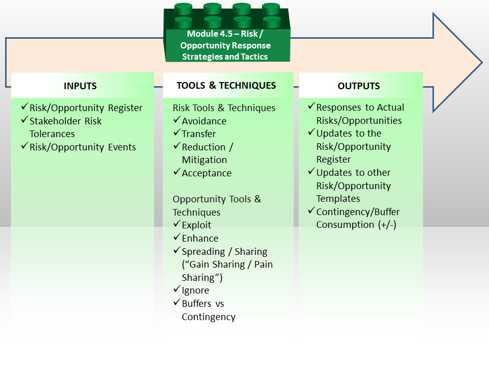
Figure 1 - The Risk/Opportunity Response Strategies and Tactics Process Map
Source: Guild of Project Controls
Referring back to the FDA process flow chart, we are now at Step 8 in their process, which the Guild has adapted by breaking the FDA Process Step 8 into two parts:
(1) Strategic Risk Response
(2) Tactical Risk Response
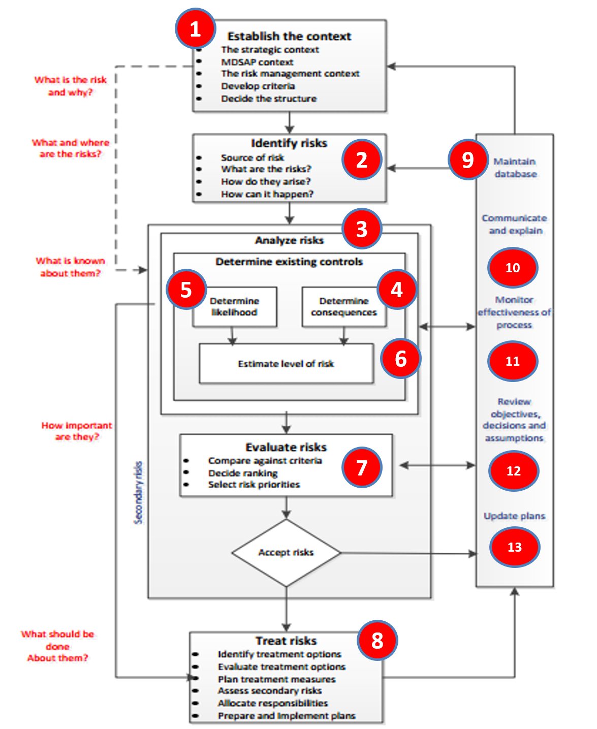
Figure 2 - US FDA “Risk Process Map” Adapted for use in the GPCCAR
Source: Guidance for Industry- Q9 Quality Risk Management (2006)
04.5.1.01 - Managing Risk
Because of the Project Controls focus on time, cost and scope objectives, only those risks and opportunities which have an effect on these objectives, are the ones that matter – those threats and opportunities which have to be identified, assessed and managed to because they affect the achievement of the planned cost, schedule and scope objectives of the project.
To support Project Controls, project risk management should therefore be primarily focused on integrating cost and schedule for a given scope of work to assess the effect of uncertainty on the time and cost objectives of the project. Such an assessment will however be meaningless unless it is stated in “the language of business” i.e. money. It is therefore the view of the author that only by quantifying the effect of risk through the application of quantitative risk analysis, can risk management provide meaningful input into risk-based project decision making and project controls processes.
While quantitative risk analysis is widely applied in diverse fields to quantify uncertainty and variability in processes, cash flows, incident rates and return on investment amongst others, the analysis of schedule and cost risk is the primary requirement of the project controls process.
Traditionally, cost and schedule risk analyses are conducted separately and most often, in isolation of each other by functionaries who rarely, if ever, consult with each other in either the initial estimation or the subsequent analysis stages. This results in widely optimistic and disparate estimates and contingency provisions.
Controlling the cost and schedule of a project is an integrated process of balancing the scope to the budget to the schedule. This realization has led to thought leaders such as the AACE formulating recommended practices as part of their Total Cost Management framework which emphasize the integrated analysis of cost and schedule (“ICSRA”) to determine the effect of uncertainty on objectives.
04.5.1.02 - Managing Opportunities
It is axiomatic that there can be no reward/opportunity without risk and hence projects are undertaken to move organizations from one strategic position to the next. It is however difficult to manage opportunities i.e. the positive side of uncertainty, as part of or a mere extension of the risk management process as it is human nature that a project team would have difficulty in considering both positive and negatives during the same risk management brainstorming session/enquiry.
Hillson (Hillson, D. and P. Simon, (2012), Practical Project Risk Management - the ATOM Methodology) has published the Active Threat & Opportunity Management (“ATOM”) method and SAVE International the Value Methodology (“VM”) Standard (SAVE, (2015), Value Methodology Standard) which is based on the well-known value engineering/analysis methods widely used in industry. VM is a systematic and structured approach for improving projects, products, and processes. VM, which is also known as value engineering/analysis, can be applied to a wide variety of applications, including industrial or consumer products, construction projects, manufacturing processes, business procedures, services, and business plans. VM helps achieve an optimum balance between function, performance, quality, safety, and cost resulting in the maximum value for the project.
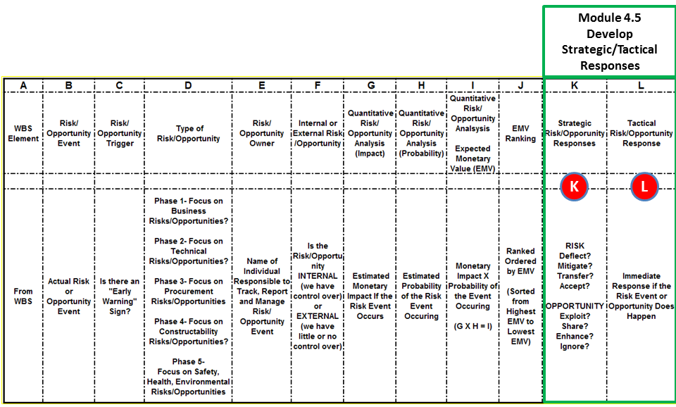
Figure 3 - Sample Risk/Opportunity Register Template Showing FDA Step 8
Source: Giammalvo, Paul D (2015) Course Materials. Contributed Under Creative Commons License BY v 4.0
04.5.1.03 - Strategic Risk / Opportunity Responses
The last two columns in our Risk Register (Figure 3 Columns K and L) are for Strategic (Figure 3 Column K) and Tactical Responses (Figure 3 Column L)
Referring back to Figure 1 we need to remember the four possible RISK response strategies are:
- Avoid
- Transfer
- Mitigate
- Accept
Likewise, for each opportunity, we also have 4 possible STRATEGIC responses to OPPORTUNITY:
- Exploit
- Share
- Enhance
- Ignore
04.5.1.04 - Tactical Risk / Opportunity Response
The final column (Figure 3 Column L) is for TACTICAL response to a risk or opportunity if it occurs.
The classic example are the first responder medical teams who arrive with an ambulance. While not full-fledged doctors they are trained medics who can stabilize a patient and keep the patient alive long enough to get him/her to a proper medical facility. This same “best tested and proven” practice needs to be adapted by the project controls team for each risk or opportunity event. Ideally, the “Risk Owner” or someone he/she has delegated has been provided with advance authority to respond immediately to a risk or opportunity before it happens (proactively) rather than after it happens (reactively). This is another aspect not commonly found in most risk registers and needs to be considered when you create one for your project or organization and will help end the perpetual “fire-fighting” mode that many project teams are constantly in. Organizations or teams in perpetual crisis management is a sign of potentially incompetent or ineffective project controls.
The Risk Owner would also be responsible to ensure that the appropriate processes and procedures have been created and that sufficient training has been conducted to ensure that “first responders” are able to react in the event a risk (or opportunity) occurs. The classic examples of this are the “first responder” training provided by nearly all major companies now. Other examples include working in restricted areas, working in areas subject to fire and explosion or people working in enclosed tanks or in trenches. While we have done a great job in terms of safety, we have not yet developed the same level of robust risk response tactics for other types of risk, i.e. Business, Technical, Procurement and Constructability.
04.5.2 - INPUTS
- RISK/OPPORTUNITY REGISTER
- STAKEHOLDER RISK TOLERANCES
- RISK/OPPORTUNITY EVENTS
04.5.3 - TOOLS & TECHNIQUES
04.5.3.01 - Tools & Techniques - RISKS
04.5.3.01.1 - Avoidance
Avoiding a potential risk event means not taking the risk in the first place. The most common example of avoidance would be using a tested and proven piece of equipment rather than picking the latest technological innovations. Many of us use this strategy in our daily lives. How? By not upgrading to the latest new operating system for at least a year after it has been released. Why? Because we know there will be bugs and better we stick with our current operating system even though it may not be perfect, we have learned to work with whatever quirks or bugs it may have.
04.5.3.01.2 - Transfer
This is the classic strategy why owner outsource work to contractor, the assumption being that the contractor is better able to manage the risk than the owner can. Unfortunately, this is often not the case as owners tend to pass along risks to contractors which the contractor is no better and in many cases less able to manage than the owner is.
04.5.3.01.3 - Reduction / Mitigation
For risks which cannot be avoided or transferred, mitigation is the best approach. With mitigation, the probability of the event happening is not diminished nor is the impact (amount at stake) What is done to protect against this kind of risk event is BUFFERS or CONTINGENCY is added as an INSURANCE POLICY that if the event does occur that time and/or money has been set aside to protect against this happening. Examples of mitigation is having a backup piece of equipment available if the primary piece breaks down.
04.5.3.01.4 - Acceptance
As explained previously, depending on the risk profile of the decision makers, there are some risks with low Expected Monetary Values which the organization is willing to accept. How “low” depends on how risk averse the decision makers are, but generally speaking those items with an EMV of <1% of the project value are generally accepted. This rule of thumb applies to both owners and contractors. (for contractors it is <1% of the contract value) Meaning that not every threat needs to be acted on. Some of them both owners and contractor’s alike are able to accept.
04.5.3.02 - Tools & Techniques - OPPORTUNITIES
04.5.3.02.1 - Exploit
As by definition an opportunity has a positive outcome, we want to take full advantage of it. The classic example is where contractors bid low on projects they feel the owner has been careless or negligent in defining scope or providing project information and they will exploit that by issuing change requests. For owners a common way of exploiting opportunity is by making bulk purchases of materials such as pipe or wire which may be used on more than one project but by buying in bulk, they can get better prices than a contractor could.
04.5.3.02.2 - Enhance
This concept is gaining more traction ever day as both owners and contractors are exploring alternate contracting methods which are less confrontational. Using these contracting methods (which will be explored in more detail in Module 5- Managing Contracts) risks are shared as are savings. These are known generically as “Gain Sharing / Pain Sharing” contracts. This is the concept underlying the various incentive contracting methods.
04.5.3.02.3 - Spreading / Sharing (Gain Sharing / Pain Sharing)
Again as an opportunity represents the potential for a positive outcome, anything we can do to improve either the probability of it being successful or increasing the savings or other benefits which accrue is why project control professionals need to know and understand this concept. Sooner or later, we will be called upon by our management to provide input into improving a schedule and / or reducing costs.
04.5.3.02.4 - Ignore
As with risks there are some opportunities that because of lack of manpower or priority (using EMV again) there is not enough potential value to be worth bothering with so we let the opportunity pass. A common example is contractors have to weigh the option of filing a claim or a change request with an owner vs how much time and money it will take to document and manage the claim. In many cases, the potential additional profit is not worth the aggravation, not to mention the bad feelings it may generate.
04.5.3.03 - Buffers vs. Contingency
See Columns K and L in Figure 3 above
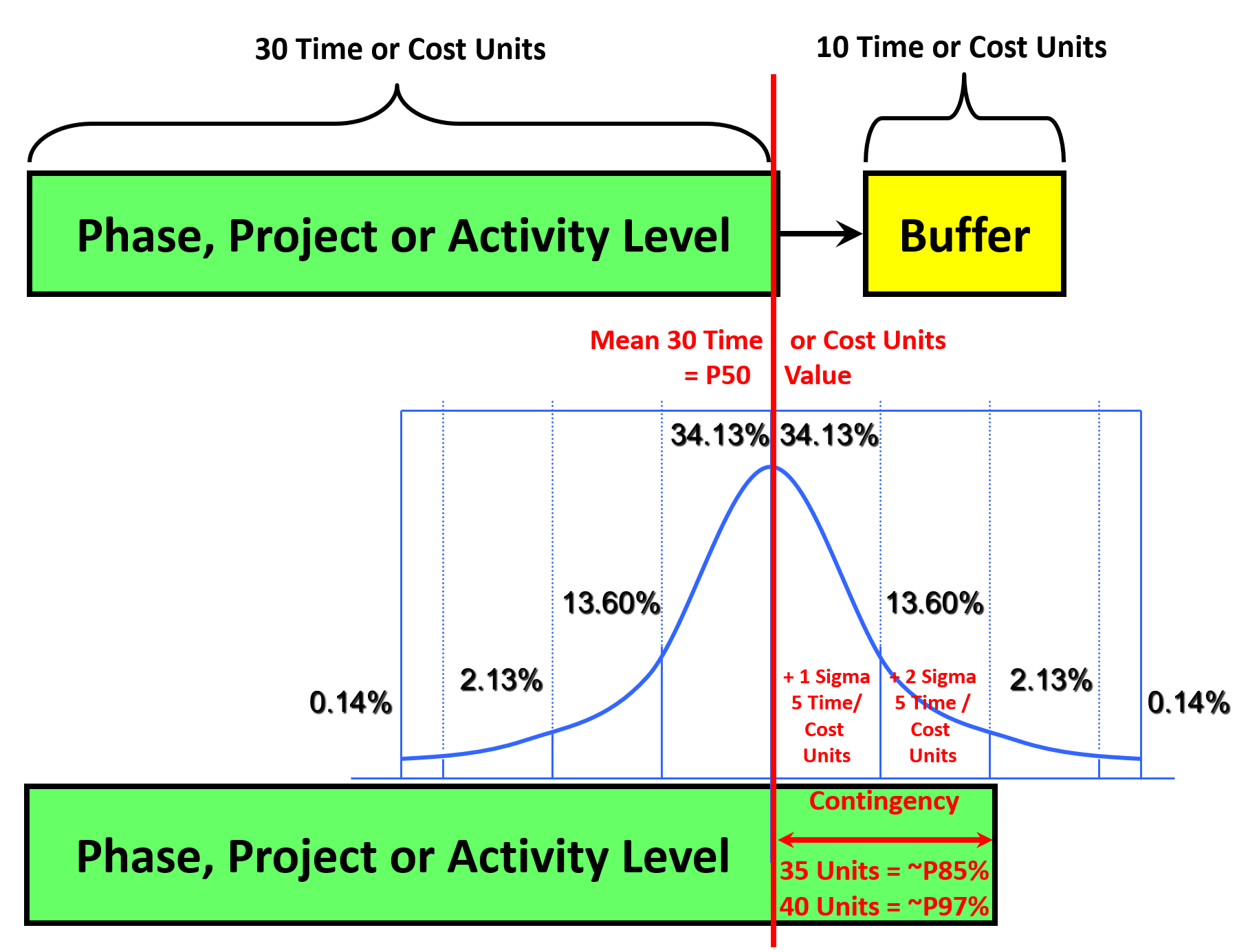
Figure 4 - Explains there are Two Approaches to Establishing Buffers or Contingency
Source: Giammalvo, Paul D (2015) Course Materials. Contributed Under Creative Commons License BY v 4.0
Both Buffers and Contingency are used to OFFSET or MITIGATE either time or cost risk which was monetized using EMV. Given that EMV can have both positive or negative values, especially as contractors, we CANNOT afford to accept a negative EMV. That means whenever we have a negative EMV that we MUST “make it go away” and the way we do that is by adding contingency (time or money) to negate or balance out the negative EMV.
See Example below under “Decision Trees” to see very clearly how contractors use this powerful tool to analyse both risks and opportunities.
While both serve exactly the same purpose, there are advantages and disadvantages that professional project control professionals need to be aware of.
Buffers come to us as a result of Eli Goldratt’s “Theory of Constraints” and as we can see from the illustration when we use buffers, we create two separate activities. The first is the P50 value and the second activity, connected finish to start is the buffer or contingency, which in this case is 10 units. While buffers work great in a production environment, by building stockpiles of materials we can shut down an segment of the operation for repairs, while keeping the production through put flowing, this concept generally does not work well in a project environment. The danger in using this is because everyone can see the activity called “Buffer”, there is a tendency for everyone in the string of activities to try to claim it as their own. Having said that, there are certain conditions (i.e. weather days) where using a buffer is an appropriate “best tested and proven” practice, but generally speaking it should be avoided unless there is a compelling argument why it should be.
On the other hand, by using the statistical method above, we can “bury” the contingency, so that only the entity putting it there (could be either the owner or contractor) is aware of it. Unfortunately, this is the reason many owners put P40 values into the contract requirements, to try to protect themselves against contractors building in hidden contingency, but as shown in the example above, if durations are unreasonably short, all the contractor does is calculate the crashing costs and the risks of not being able to do it in the owners time frame and then passing the costs of that risk along to the owner in the form of higher prices.
Case Study Illustrating the use of Buffers/Contingency
- For calculation purposes, let’s assume a day is worth $10,000. And let’s assume that Task 7 shown above is on the critical path. We can see that the mean or “P50” value for this activity is 10 days and we can see that the sigma or standard deviation is 1.1 days. We can also see that the variance (1.1^2/2 = .605 days) falls within our +/- 3 sigma rule of thumb, meaning this is NOT a risky activity.
- Now the question becomes what is the RISK PROFILE of your stakeholders? If they are risk seeking, they may be willing to establish the planned duration at 8 days which according to the simulation only has a 5% probability of being achieved, understanding that means there is a 95% probability it will take longer than 8 days. IF this is the case, then the difference between P50 (10 days) and the P05 duration of 8 days is -2 days x $10,000 per day = (-$20,000) This helps explain why the green curve in Figure 4 above increases as we try to crash the activity and how to calculate the impact crashing has. This is NOT a good practice although it is a very common one used by owners to try to push contractors to perform work faster. By understanding this set of calculations, owners need to understand that all the contractor has done is monetize the risk that it will take 10 days not 8 and has passed on the costs of crashing to the owner in the form of higher prices.
- Let’s assume the stakeholder is risk averse and chooses 12 days, which gives us a P95 meaning there is a 95% chance the activity will take LESS than 12 days and only a 5% chance it will take more than 12 days. Now we have a P50 value of 10 days and $10,000 X 10 = $100,000 risk value for this activity. By adding two more days, we have now built in a BUFFER or CONTINGENCY of 2 days and 2 days X $10,000 = $20,000.
Explained another way CONTINGENCY is the difference between the P50 or mean value and whatever P level management has chosen. And that the contingency or buffer can have either a positive or negative value. If it is a negative value, the contractor passes the cost of that event along to the owner in the form of higher prices in exchange for accepting the costs associated with crashing and if it is a positive value the entity that established it is the own who owns and controls it. This will be explained in more detail in Module 7- Managing Planning and Scheduling and Module 8 - Managing Cost Estimating and Budgeting, but for the time being, recognize this is a risk mitigation tool and technique that has broad applications especially in the PS and CM tracks.
04.5.3.04 - Decision Trees Using Expected Monetary Value
Decision Trees are another common risk analysis tool/technique to help us visualize our strategic and/or tactical options in order to help us make better, more informed decisions based on facts and not emotions or gut instinct.
The best way to demonstrate how Decision Trees work is to provide a simple case study which is based on how contractors MONETIZE risks placed on them by owners and pass those monetized risks back the owner in the form of higher prices.
Decision Tree Case Study
Below is an actual example showing how contractors use Decision Trees combined with Expected Monetary Value (EVM) to analyse and mitigate Risk and enhance Opportunity.
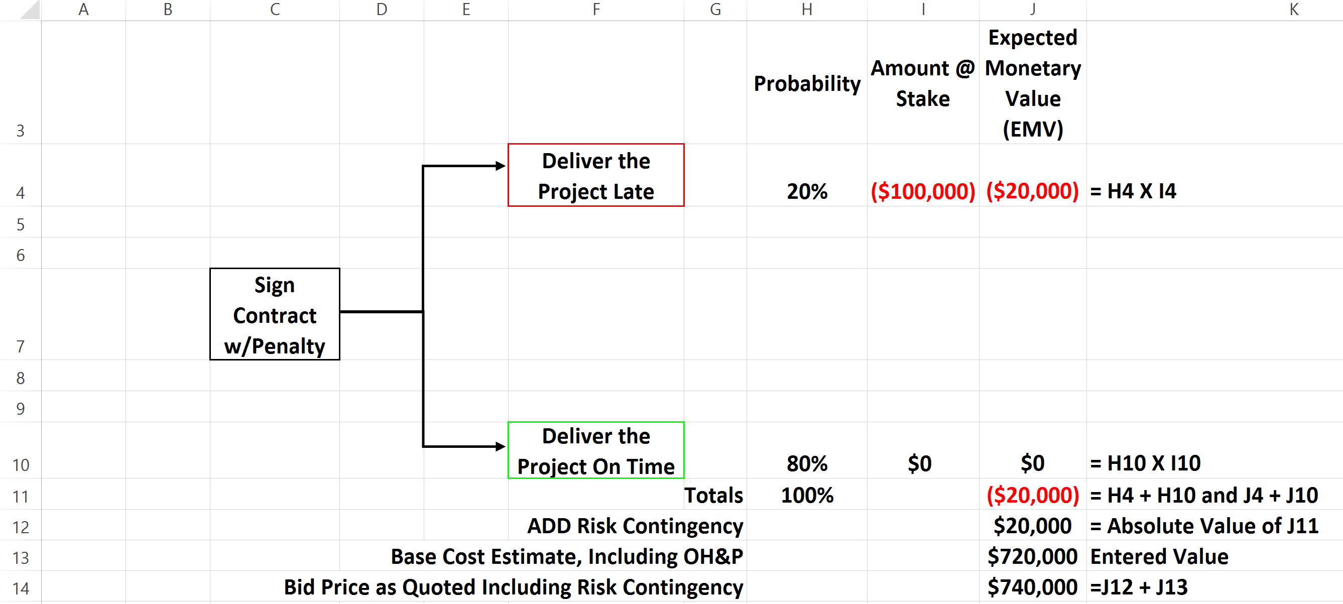
Figure 5 - Scenario One- Penalty Clause Contract Only
Source: Giammalvo, Paul D (2015) Course Materials. Contributed Under Creative Commons License BY v 4.0
- In the scenario above, the owner has issued a contract which has a $100,000 late delivery penalty clause. (For simplification it is only a flat penalty, not per day) The contractor (using past history combined with expert opinion) determines that he has a 20% chance of finishing later than the contractual date and an 80% probability of finishing on/before the contract mandated completion date.
- To calculate the “premium”(impact or consequence) of the risk he will finish late, the contractor multiplies 20% probability of finishing late X $100,000 late delivery penalty which yields an EXPECTED MONETARY VALUE of ($20,000)
- He also multiplies the 80% probability of finishing on time X the BONUS which in this scenario, is $0.00 which of course, yields an EMV of $0.00.
- Then when he adds up the EMV of both potential options he ends up with a NEGATIVE EMV of ($20,000)
- Because no contractor who wants to stay in business is willing to accept a negative EMV, he has no choice but to add a RISK CONTINGENCY of $20,000 to offset the negative EMV potential of incurring a late delivery penalty. The contractor then calculates his bid price of $720,000, add to it the risk contingency of $20,000 and his RISK ADJUSTED BID now becomes $720,000 + $20,000 = $740,000.
What owners need to understand is that every RISK they put on the back of the contractors, the contractor MONETIZES that risk and passes it back in the form of HIGHER PRICES. So in this case, congratulations Mr. Owner, you have not penalized the contractor at all. All you have done is raised the cost of your project as the contractor monetized the risk of your late delivery penalty and passed it back to you in the form of higher prices…
In our next scenario we see that a more enlightened owner has added a BONUS option along with the PENALTY. (Offering both a carrot and a stick)
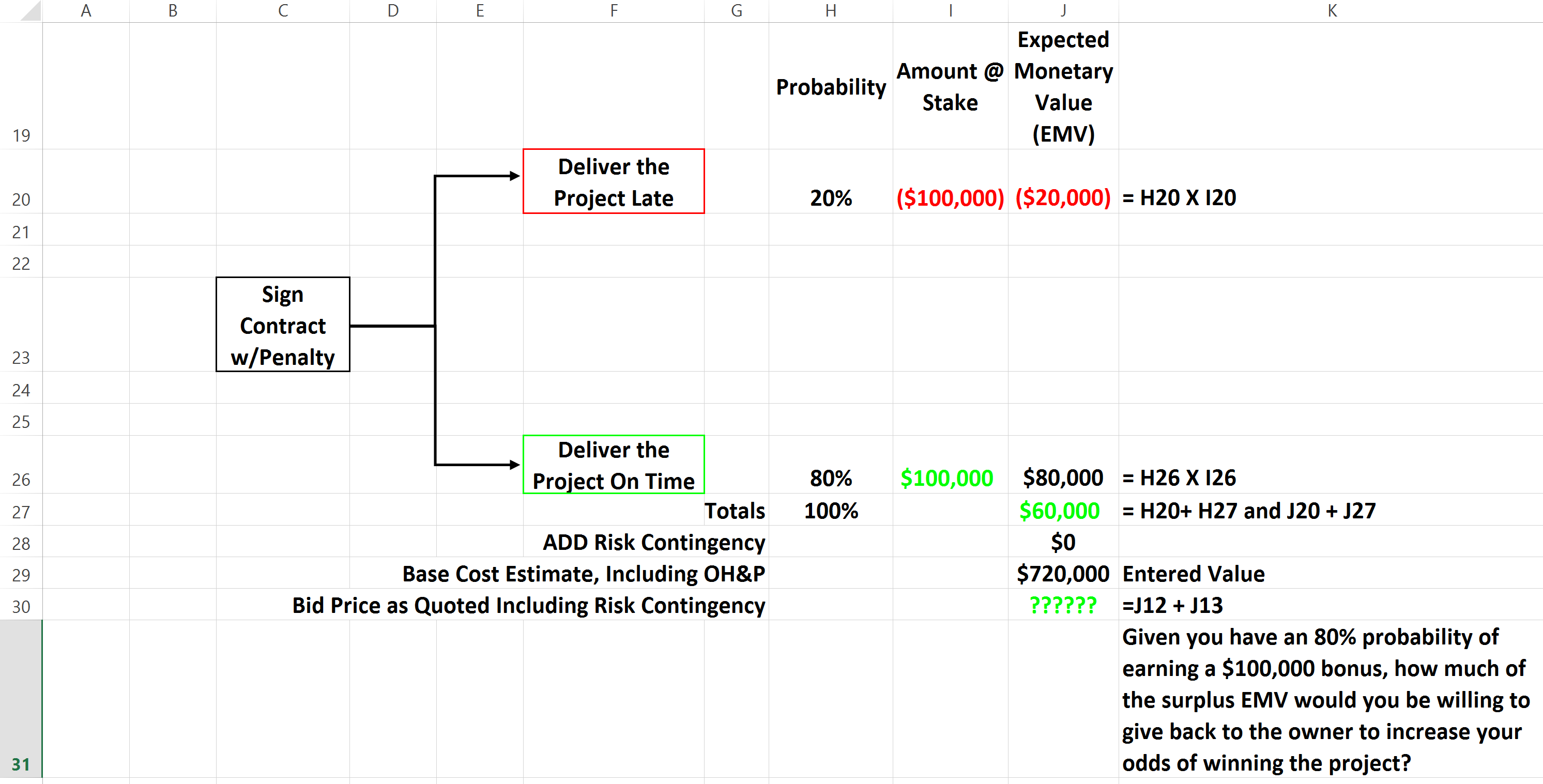
Figure 6 - Scenario Two- Penalty and Bonus Clause Contract
Source: Giammalvo, Paul D (2015) Course Materials. Contributed Under Creative Commons License BY v 4.0
In the second scenario, we can see that by adding the opportunity to earn a BONUS of $100,000, 80% X $100,000 = +80,000 EMV and adding the ($20,000) EMV = +$60,000 POSITIVE EMV.
- Now, given the contractor has negated his risk and still has a $60,000 surplus EMV, and knowing that he has an 80% probability of earning a $100,000 bonus, and that for each dollar he lowers his price INCREASES his odds of winning the bid, the question is how much of that $60,000 would he be willing to LOWER HIS BID (effectively giving back some of the bonus money to the owner) in order to increase his odds of winning the bid?
This is a perfect example of how Decision Trees and EMV are used as a tool & technique to quantify, analyse both risk and opportunity in order to develop viable risk and opportunity strategies.
04.5.4 - OUTPUTS
- RESPONSES TO ACTUAL RISKS/OPPORTUNITIES
- UPDATES TO THE RISK/OPPORTUNITY REGISTER
- UPDATES TO OTHER RISK/OPPORTUNITY TEMPLATES
- CONTINGENCY/BUFFER CONSUMPTION (+/-)
04.5.5 - REFERENCES & TEMPLATES
- National Defense Industrial Association (Ndia) (2014 Integrated Program Management Division “A Guide To Managing Programs Using Predictive Measures Http://Www.Ndia.Org/Divisions/Divisions/Ipmd/Documents/Workinggroups/Predictive_Measures_Guide_Ipmd_Review_Copy.Pdf Page 64
- National Defense Industrial Association (Ndia) (2014 Integrated Program Management Division “A Guide To Managing Programs Using Predictive Measures Http://Www.Ndia.Org/Divisions/Divisions/Ipmd/Documents/Workinggroups/Predictive_Measures_Guide_Ipmd_Review_Copy.Pdf Chapter 5
- US Federal Aviation Administration Risk Management Handbook (2009) Http://Www.Faa.Gov/Regulations_Policies/Handbooks_Manuals/Aviation/Risk_Management_Handbook/
- NASA Risk Management Handbook (2011) Http://Www.Hq.Nasa.Gov/Office/Codeq/Doctree/Nhbk_2011_3422.Pdf
- Jardine, Scott Pricewaterhousecoopers (2007) Managing Risk In Construction Projects Http://Www.Pwc.Co.Uk/Assets/Pdf/Pwc-Cps-Risk-Construction.Pdf
- University Of Adelaide (N.D.) Risk Management Handbook- Http://Www.Adelaide.Edu.Au/Legalandrisk/Docs/Resources/Risk_Management_Handbook.Pdf
- US Dept Of Transportation (2013) Transportation Risk Management: International Practices For Program Development And Project Delivery Http://International.Fhwa.Dot.Gov/Scan/12030/12030.Pdf
04.6 - Module 04-6 - Risk / Opportunity Monitoring and Control
GPCCAR M04-5 - Risk & Opportunity Response Strategies and Tactics, Revision 1.00