M09-5 Project Performance Forecasting

09.0 - MANAGING PROJECT PROGRESS

09.1 - Module 09-1 - Introduction to Managing Project Progress

09.2 - Module 09-2 - Develop the Managing Project Progress Policies & Procedures Manual

09.3 - Module 09-3 - Capturing Progress & Updating the Schedule

09.4 - Module 09-4 - Assessing & Interpretting Progress Data

09.5 - MODULE 09-5 - PROJECT PERFORMANCE FORECASTING

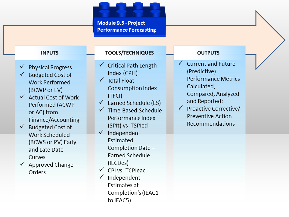
Figure 1 - Project Performance Forecasting Process Map

Source: Guild of Project Controls

09.5.1 INTRODUCTION

In the previous Module 09.4 - Assessing and Interpreting Progress Data, we were focusing on the past to the present to help us understand what was happening on our project.  Now it is time to look forward to see where todays status is taking us; Forecasting.

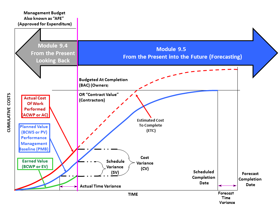
Figure 2 - Curve Showing Focus of Module 9.4 Assessing & Interpreting Progress & Module 9.5 Project Perofrmance Forecasting 

Source: Adapted from DAU Gold Card KPI’s, 2015

As we can see from the above graphic, in Module 9.4 we focused on the past up until the present (evidenced by the “Time Now” or “Data Date” line), because this was past history with sunk costs while it was easy to see if our project was headed for trouble, there was little if anything we can do to fix any problems identified.

• But now that we’ve switched focus from the past up to the present and are now using Earned Value Management tools & techniques to look into the future, the expectations are that we now can be more proactive about making the kinds of decisions to fix the existing problems (if any) and to try to prevent others from happening.

While it is important for project controllers to be able to reconstruct what happened in the past, especially those doing forensic analysis, the real value that project controls professionals can make is being able to use past performance as the basis to predict what is likely to occur in the future, with the objective to be able to be proactive, making adjustments to the productivity, manpower or other variables to ensure that the project finishes within budget and on time.

The simple analogy is driving your car down the road. One cannot drive forward by looking in the rear view mirror.

The only way one can drive safely and get where we are going is by looking forward and continually making corrections in our speed, best traffic route and fuel efficiency to reach our destination on time and within the fuel and cost budget allocated.

Explained another way, project controls is to project management what your GPS Tracker is to driving your car, especially in a new city.

Once we start to understand our roles as project control professionals in that context, it makes a lot more sense in helping understand and appreciate what information our clients and other stakeholders need and want from us and also just as relevant, is how they need and want to be receiving this information.

As professional practitioners, we live in a mobile technology world and the faster we can adapt our data collection and data analysis and communications using mobile devices, the more respected and appreciated we will become.  Refer Figure 3 - Magellan Smart GPS on the right (Source: Magellan GPS Systems).

09.5.2 INPUTS

• Physical Progress
• Budgeted Cost Of Work Performed (BCWP or EV)
• Actual Cost Of Work Performed (ACWP or AC) From Finance/Accounting
• Budgeted Cost Of Work Scheduled (BCWS or PV) Early And Late Date Curves
• Approved Change Orders

While the inputs for both modules are largely identical, it is the tools & techniques which change considerably, moving from a backwards looking focus to a forward looking focus, using forecasting techniques.

09.5.3 TOOLS & TECHNIQUES

As with all the tools and techniques shown below, there are simply too many variables to tell you which tool should be used in any given circumstance. It is up to you as a professional practitioner to KNOW and UNDERSTAND how to use each of these tools and techniques and in the event you are unsure which one is “better” or “best” in any given circumstance it is up to you to seek out advice from your supervisor or mentor.

09.5.3.1 CHECK SCHEDULE ACCURACY, ASSESS MILESTONES & COMPLETION DATES

09.5.3.1.1 Confirm Schedule Accuracy With Site Teams Plan

Up to this point, we have updated the schedule with progress and cost information, run all the diagnostics for both time and cost, looking not only at the current date backwards (forensic analysis) but more importantly, from the current date looking forward (forecasting).

• We now need to focus on potential corrective actions, which means either accelerating the schedule (crashing, fast tracking or descoping) or accepting that the project will be late and which means rebaselining the schedule to reflect the revised completion dates.

For those working on new product development projects (e,g, IT, Pharmaceuticals or Telecommunications) where being “first in the market” means the difference between capturing the majority of the market share, it also means a delay in the completion of the project by only a few days, weeks or months may significantly impact the business case, meaning a forecast delay may cause the project to be cancelled or significantly modified.

• The contractor checks that the site team are working to the plan, that the schedule is accurate and that the schedule still reflects how the site team believes the works can be implemented.

The next step is to validate that the interim milestones and the completion date remains per the approved baseline and if not where are the variance’s (plus or minus).

09.5.3.1.2 As Built vs As Planned Schedule

The two examples below illustrate a typical “As Built” vs “As Planned” schedule.

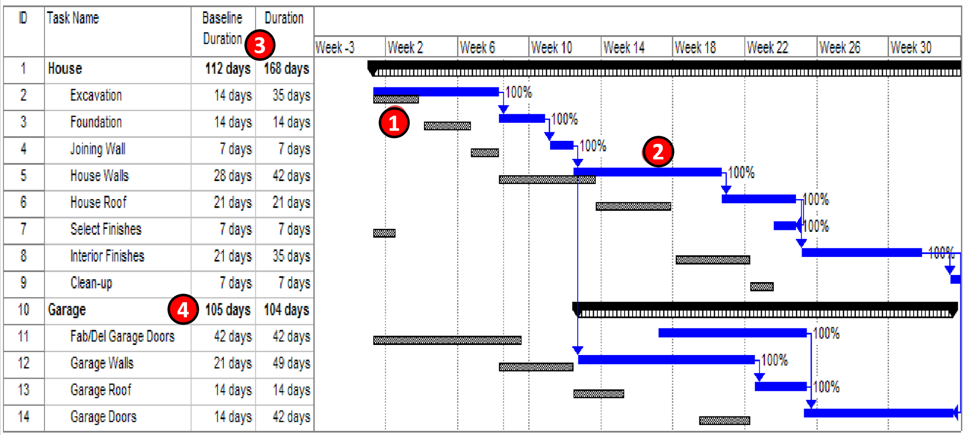
Figure 4 - “As Planned” vs “As Built” Bar Chart schedule

Source: Lazarczyk, Jack A. CPA, CCC, (2003)

As we can see, the original baseline is represented by the grey bars (1) while the current “as built” schedule the activities are shown in blue (2). What this tells us is that the HOUSE (3) is running 168-112 = 56 days behind schedule (negative float) while the garage (4) is running 105-104 = 1 day AHEAD of schedule.

• While this is a very simplistic example, it provides the essence of how to use this tool to compare the as built to the baseline schedule.

BUT, there is a whole lot more we can do to analyse the overall health of our projects besides just using the bar or Gantt Chart views. Another of an “As Planned” vs “As Built” schedule, but instead of showing the activity bars, the delay was actually calculated and shown on the schedule.

Both methods are commonly used but the first one is probably the one most commonly seen.

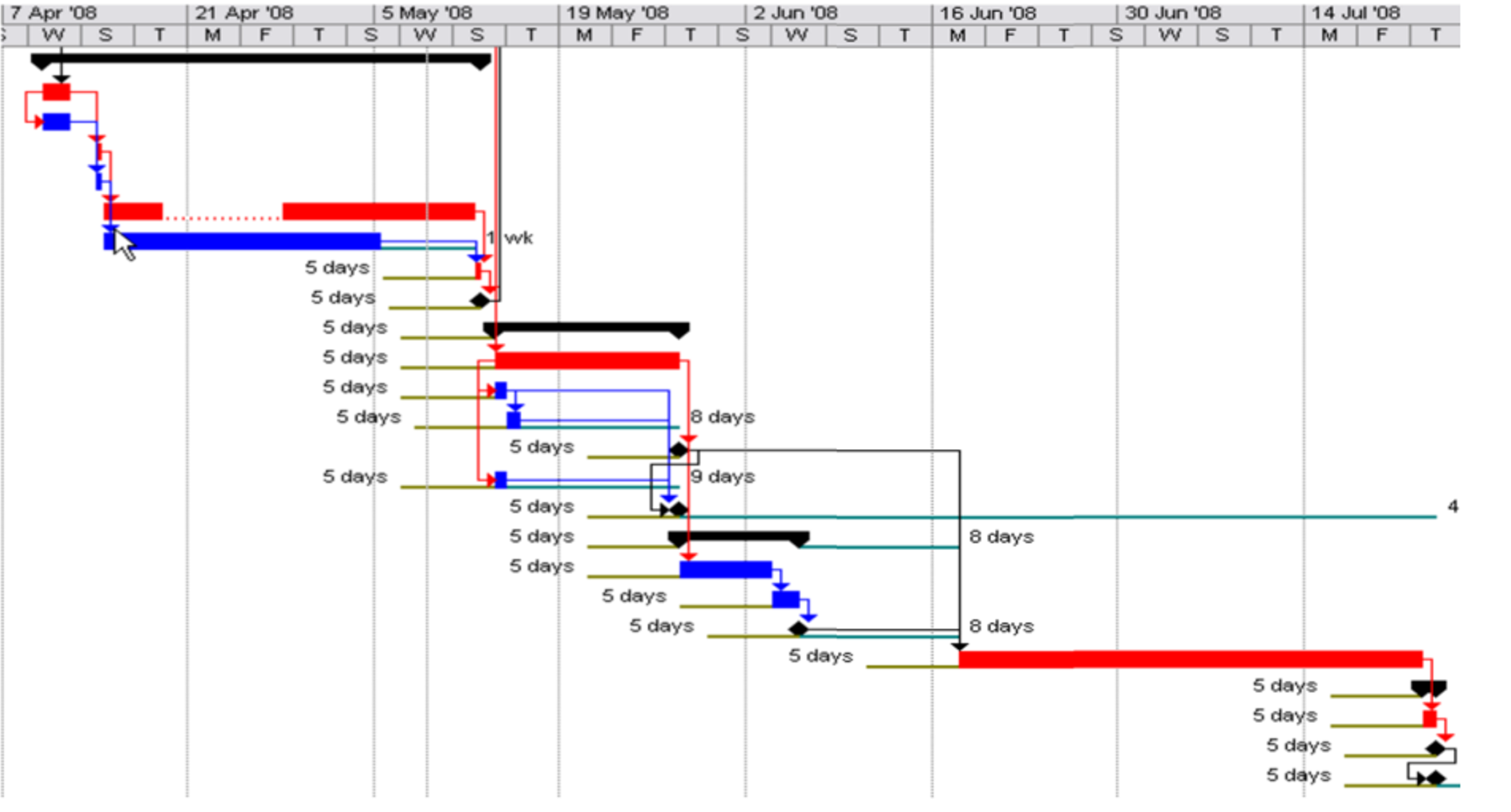
Figure 5 - As Planned vs As Built comparison

Source: Construction Impact Analysis (n.d.)

As we can see from two graphics above, the blue activities are not critical while the red activities are critical while the lines, which are coming from the original or updated baseline indicate how much each activity has slipped.

As explained in Module 7 - Managing Planning and Scheduling, there are only 4 possible options to address this situation:

1. Ignore it- and the project is going to finish at least 5 days late
2. Crash the critical path activities- by ADDING more resources with the hopes we can recover those 5 days. Because crashing invariably raises the cost of the project, in addition to only crashing activities which are critical, we also need to select the activities which give us the most schedule compression for the least amount of money.
3. Fast Tracking- maybe it is possible that instead of Finish to Start, we can change the logic to show Start to Start with a lag or Finish to Finish with a lag?
4. Descope- while not always possible, in many cases, especially bringing new products to market (i.e. software) it is common to delete some features or functions in order to get the project to market faster, knowing that the missing features or functions will be added when the next update is released.

09.5.3.1.3 Adding Activities to the CPM Schedule

Very often we find that either because scope was forgotten and we find a new activity has to be added or there was an approved variation / change order or there was an identifiable cause for a delay, often we need to add additional activities.

Using a simple frag-net for constructing GSM Communications Tower sites as an example, we will demonstrate how to add activities correctly.

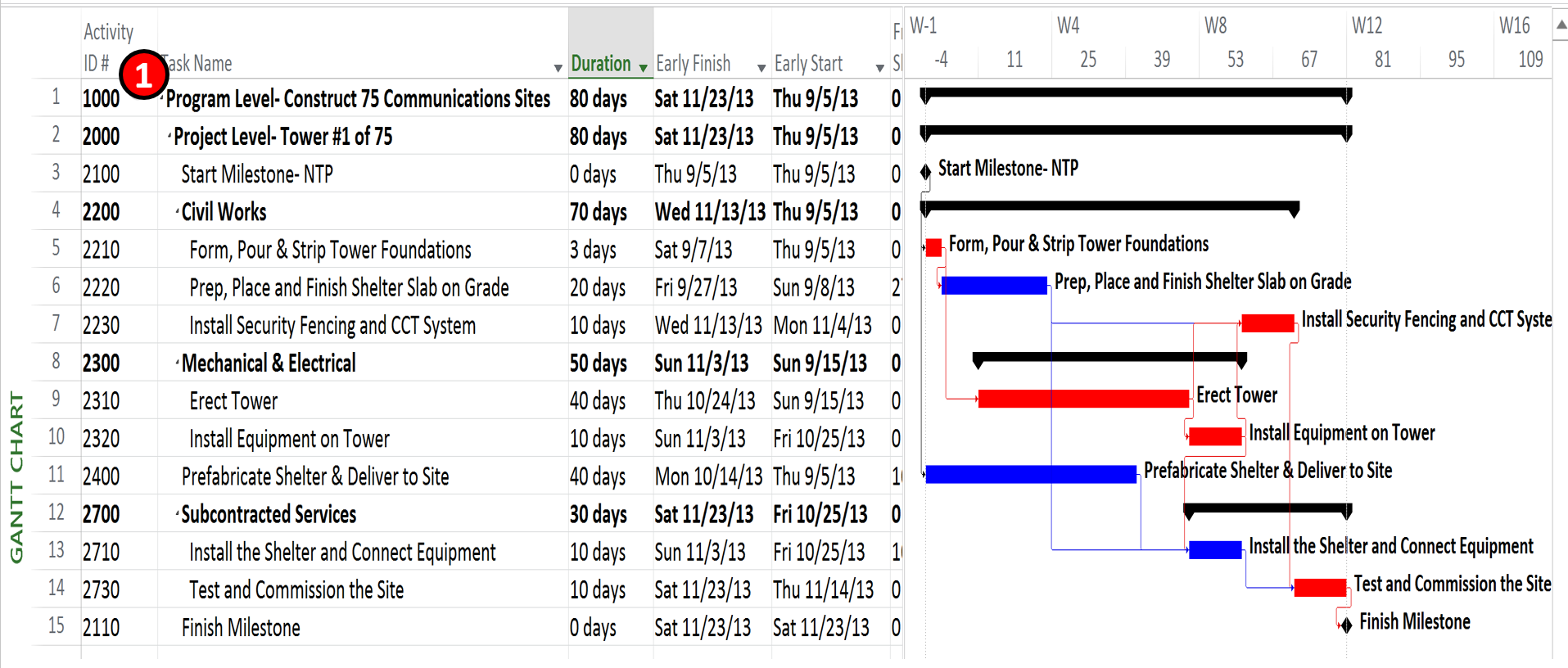
Figure 6 - Frag-net Schedule for a single GSM Communications Tower Site

Source: Giammalvo, Paul D (2015) Course Materials Contributed Under Creative Commons License BY v 4.0

As explained in Module 7 - Managing Planning and Scheduling, Activity ID’s (1) should be kept as simple as possible and not contain extensive or elaborate coding structures. If we want to sort and filter, it is preferable to use the various sort fields or any of the customizable sort fields. It is also important to leave plenty of space in between the initial activity ID numbers, anticipating that at some point, you will have to add more activities.

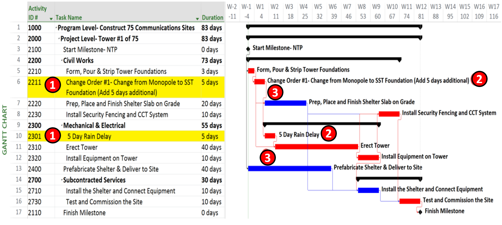
Figure 7 - Showing how to ADD Scope Change and Delay Activities to the Schedule

Source: Giammalvo, Paul D (2015) Course Materials Contributed Under Creative Commons License BY v 4.0

1. Activity ID #- By keeping simple Activity ID codes and leaving plenty of space between the numbers it is easy to insert new activities. If you want to get fancy, then use only EVEN numbers for the original baseline schedule and use ODD numbers for all change orders and delays.
2. Be sure to be clear in NAMING the activity whether it is a CHANGE or a DELAY. Ideally, you should reference the Change Order Number either in the Activity Name or in the “Notes” field.
3. Whenever you add in a CHANGE ORDER or a DELAY, leave the ORIGINAL logic in place and ADD the new or revised logic. This makes it a lot easier for the forensic analysts to be able to see what happened without having to compare two different schedules to see what changes were made.

09.5.3.1.4 Reporting New Activities Introduced to the CPM Schedule

Lastly, it is important to be able to see the impact that adding scope changes or delay costs has on the Early and Late Date S Curves, as you will surely need to be able to explain it to your clients and stakeholders via the project reporitng regime.

As noted above, this information would normally be coming to the owner’s project control team from the contractor’s project control team and while any changes to the baseline (logic, changes in activities, adding or deleting activities etc) should be clearly identified and explained by the contractor in their narrative or transmittal cover letter, it remains up to the owner’s project control team to conduct their own “due diligence” on the schedule and not simply “rubber stamp” it as being accepted. Refer back to Module 4- Managing Contracts and it is entirely possible for an owner to unwittingly (by the actions of the parties) “approve” a change order by accepting a schedule which contains logic, durations or additional changes.

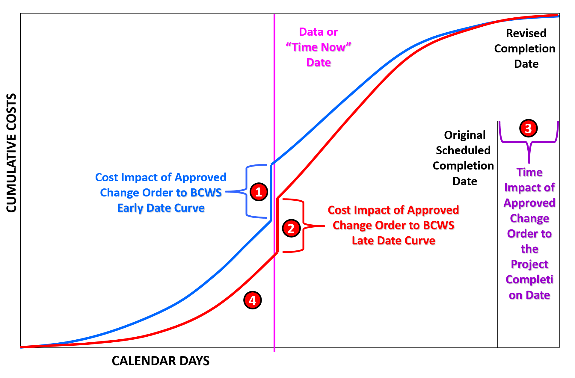
Figure 8 - Showing the Impact Change Orders and Delays have on the “S” Curve and Completion Dates

Source: Giammalvo, Paul D (2015) Course Materials Contributed Under Creative Commons License BY v 4.0

In the above example, we can see that:

1. When we add in ADDITIONAL activities which have been properly cost and resource loaded or add in the cost of DELAYS (i.e. Standby Time) it causes a JUMP in the shape of the S Curves. This should be shown in the reporting period when the Change Order was APPROVED or the DELAY was incurred. While in this case, as the change order and delay were ADDITIVE, it caused the cumulative cost of work scheduled to INCREASE, but it could have also been a SUBTRACTIVE change, in which case the cumulative BCWS would have DECREASED.
2. Because the only difference between the S Curves is the Early Date Curve activities are scheduled to Start AS SOON AS POSSIBLE (ASAP) and the Late Date Curve the activities are scheduled to start AS LATE AS POSSIBLE (ALAP) the size of the increase will be identical.
3. We can also see the impact of the CHANGE ORDER or DELAY on the Contractual Completion Dates as well. When this occurs, the owner may accept the delay in which case the schedule would be REBASELINED or the Owner may ask the contractor to prepare a RECOVERY SCHEDULE showing how the contractor can crash or fast track the remaining work to finish per the original contract completion dates.
4. Important to note and understand is that when the Cumulative Value of the project (the BAC or Contract Value) has INCREASED, because the base is now higher than it was before the delay or change order, that means the BCWP (Earned Value, shown in green above) is now being compared against a larger base, thus the PHYSICAL PERCENT COMPLETE will DECREASE.

09.5.3.2 SCHEDULE METRICS

There are a total of 5 “forward looking” Schedule Metrics and 5 “forward looking” Cost Metrics for a total of 10 which are direct derivatives of the basic Earned Value calculations introduced in Module 7-11 - Baselining & Communicating the Schedule and Module 08-10 - Baselining And Communicating The Cost Estimate/Cost Budget.

More information can be found in the NDIA’s Guide to Managing Programs Using Predictive Measures (2014) but a brief explanation of each tool has been incldued below.

09.5.3.2.1 Critical Path Length Index (CPLI)

The formula for the Critical Path Length Index is:

• CPLI = (CRITICAL PATH LENGTH + CRITICAL PATH TOTAL FLOAT)/CRITICAL PATH LENGTH

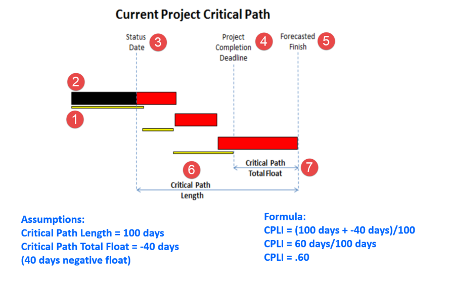
Figure 9 - NDIA Example for CPLI with numbers added

Source: Guide to Managing Programs Using Predictive Measures (2014) NDIA

To calculate and analyse the critical path using the Critical Path Length Index (CPLI) we need to know

1. The original or current baseline for the project (shown as small bars)
2. The current progress (large bars) compared against the Baseline
3. The “Time Now” or “Data Date” line
4. Original or Target Project Completion Date
5. PROJECTED Project Completion Date
6. Critical Path Length which is the difference between the Data Date and the current scheduled completion date.
7. Critical Path Total Float, which in this case is a NEGATIVE value- that is, we are finishing AFTER the finish date defined in the original baseline schedule.

• Why do we calculate this and how or why do we use it?

Depending on the stakeholder, talking about “negative float” or “positive float” is considered to be jargon and thus can cause confusion. So to make it more understandable, we use what amounts to an efficiency factor which measures or assesses the relative risk of the project finishing before, on or after the scheduled completion date. Thus the CPLI measures how efficiently we are performing against the baseline schedule. If the number is >1 then we are beating the schedule (opportunity) and if the number is <1 then we are going to be late (risk event).

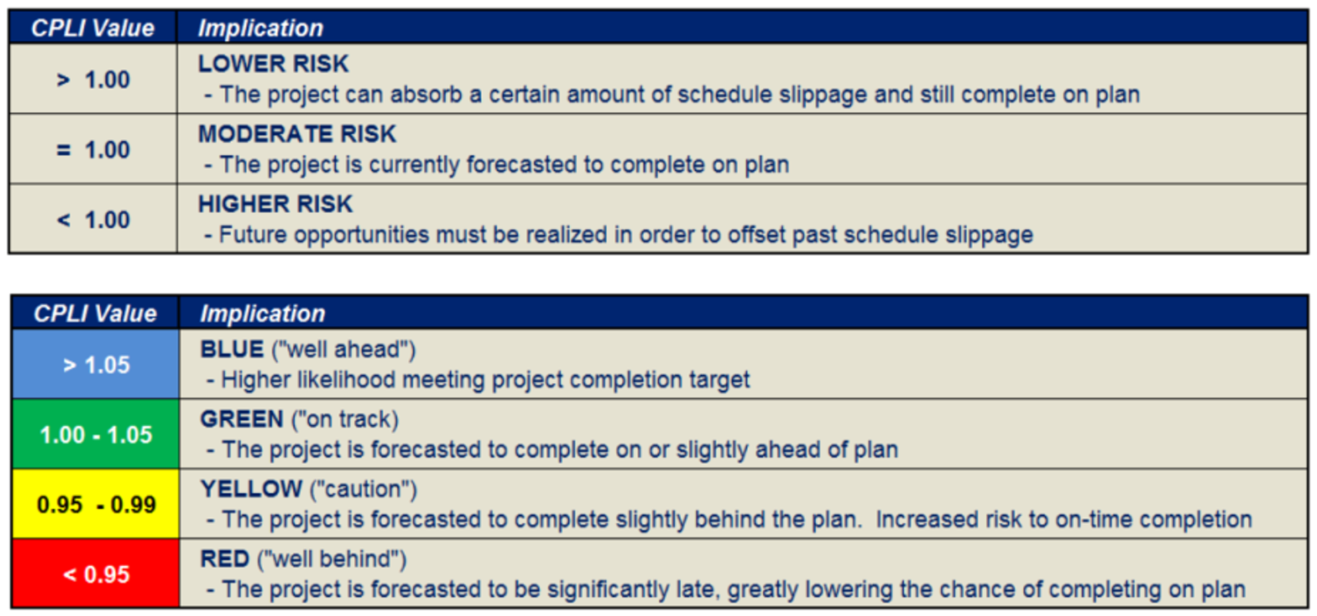
Figure 10 - NDIA CPLI Analysis Metrics

Source: Guide to Managing Programs Using Predictive Measures (2014) NDIA

09.5.3.2.2 Total Float Consumption Index (TFCI)

To use the Total Float Consumption Index is a two-step process. First we need to calculate the TFCI. The formula for that is:

• TFCI = (Actual Duration + Critical Path Total Float)/Actual Duration 

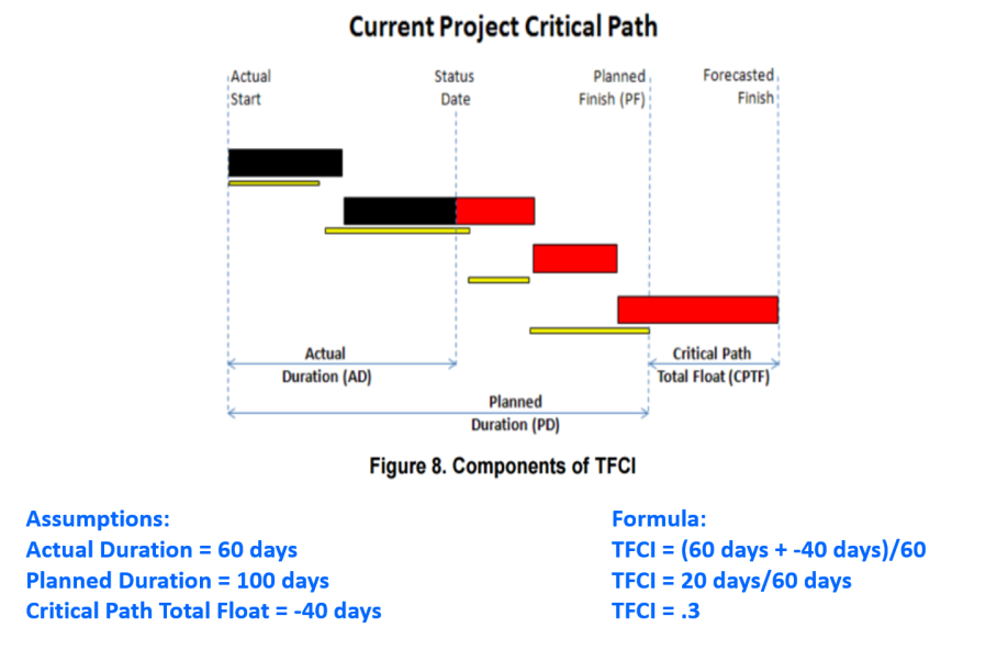
Figure 11 - TFCI factor 

Source: Guide to Managing Programs Using Predictive Measures (2014) NDIA

Once we have the TFCI factor, we can then calculate the predicted Independent Estimated Completion Date (IECD) of the project based on the current TFCI.

• What the TFCI tells us is how quickly we are eating up our float.

As an example, if we are working 22 days a month and last month we had 44 days of total float and this report period we find we have only 15 days of total float, that means we “ate up” 44 – 15 = 29 days of total float in only 22 working days. Explained another way, we are consuming float at the rate of MORE than one day of float per working day. (29/22 = 1.32 days of float “lost” for each working day).

Clearly this is not sustainable and serves as yet another “early warning” sign of problems (risk events) which are likely to happen in the future. By using the TFCI as shown below, we can use it to predict when the project is likely to finish UNLESS we identify the root causes and initiate corrective actions. 

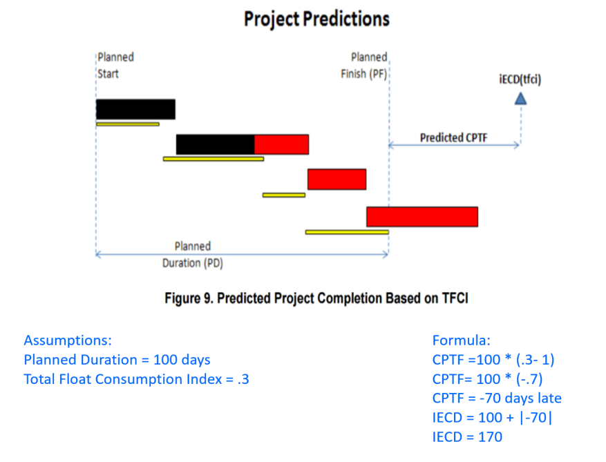
Figure 12 - NDIA Example of TFCI and IECD 

Source: Guide to Managing Programs Using Predictive Measures (2014) NDIA

• Explained another way, what this is telling us is that if we have 40 days negative float at the end of 60 days, and the planned finish was 100 days, that unless we make some big changes, we will have an ADDITIONAL 30 days of negative float at the end of the project for a total duration of the 100 days originally planned PLUS 70 days of negative float.

Unfortunately, this appears to be an all too common occurrence, which is why today’s project control professional needs to know and understand how to apply this formula.

09.5.3.2.3 Earned Schedule (ES)

The concept of earned schedule was once somewhat of a contentious issue, particularly amongst older, more experienced practitioners who have been using earned value since the 1960’s but is now more widely recognised and adopted within the ISO 21508 EV standard and Australian Standards for Earned Value.  

Earned Schedule or Earned Time is essentially a subset of Earned Value.

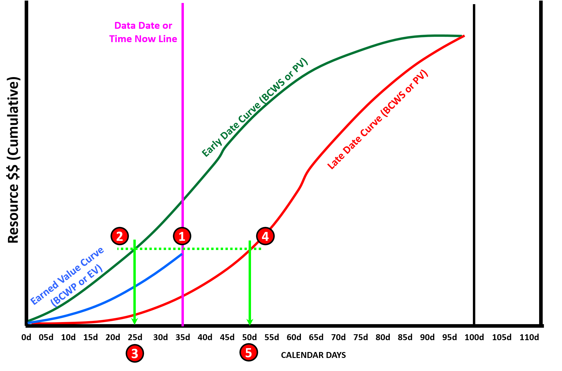
Figure 13 - Showing Both Early and Late Date Curves with the Float Analysis Illustrated 

Source: Adapted from Humphrey's Gary (2015) Project Management Using Earned Value, 3rd Edition

The concept of “earned schedule” is based on the formula to turn the Schedule Variance into time. While many “old timers” believe this has always been part and parcel of Earned Value, it was “rediscovered” by our some of our more recent IT colleagues popularizing what many of us in construction believed was always a core element of Earned Value dating back to the 1960’s.

In the example above, we can see that while the current data date is Day 35 (1), by drawing a horizontal line from where the BCWP curve intersects the Time Now or Data Date, to where that horizontal line intersects the early date curve, (2) we can see that we really have only “earned” 25 (3) days’ worth of work. Explained another way, as of day 35 we are where we should have been back on day 25, meaning we are 10 days LATE IF we wanted to hit the early date curve. Likewise, if we look to see where the same horizontal line intersects the late date curve, (4) we can see that we have “earned” 50 days (5) or are 157 days ahead of schedule vs the late date curve. The key point being comparing where we are against ONLY the early date curve (which tends to be overly optimistic to start with) only tells us part of the story. What is most important is that we stay between the two curves and don’t start drifting towards the late date curve.

As with costs, we can use a number of “earned schedule” formulas to predict the future completion date of the project. These formulas are shown below. What is important to recognize is that the truly competent project control practitioner has to apply sound professional judgement to determine which of the formulas below is the “best” or “most appropriate” to use in any given situation. The reason being is depending on the formula used, the predictive results can vary considerably and selecting the “wrong” or inappropriate formula can result in either overly pessimistic or overly optimistic results.

Which is why, unless we can clearly identify and justify the use of one formula over another, the “safest” way is to use the outcomes and from them, pick a “best case” value, a “worst case” value and a “most likely” value then applying the PERT formula, (see calculate the Mean, the sigma or standard deviation and then ask the client, sponsors or key stakeholders what “P” or “comfort level” they want and calculate the predicted finish date using that approach. Keep in mind that the higher the variance the more risky the calculations so whenever there is a large variance it is advisable to pick a higher “P” or “confidence” level. (i.e. If the stakeholders picked P90 and the variance was large, then the wise project control professional would recommend they use P95 or P98).

09.5.3.2.4 Time-Based Schedule Performance Index (SPIt) vs TSPIed

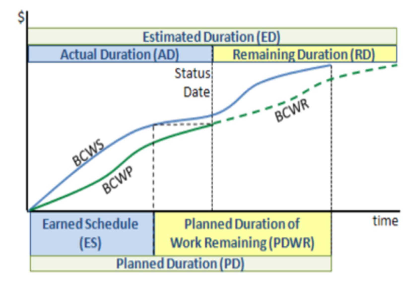
Figure 14 - Time Based Schedule Performance Index (TBSPI) 

Source: Guide to Managing Programs Using Predictive Measures (2014) NDIA

Using the data from the above example (which is actually the “better” way to show it than the example in the NDIA document which only uses the early date curve) we can see that based on the EARLY DATE curve our SPIed is Earned Schedule (25)/Actual Duration (35) or ~0.71 efficiency factor.

Given that our Planned Finish Date is day 100 our projected Early Date finish using “earned schedule” is (100-25)/.71 = ~day 106 or 6 days later than planned.

If we apply the same formula to our SPIld curve, we can see that we have earned 50 days against the late date curve, meaning 50/35 = 1.43.

As there are 106-35 days left in the revised schedule, 71/1.43 = 50 more days working at the current late date efficiency factor.

50 days’ worth of work remaining plus 35 elapsed puts our late date finish at day 85.

In other words, working to the late date curve, it is mathematically possible to finish earlier than trying to work to the early dates.

This is where sound professional judgement of the project control practitioner needs to be applied to see which formula makes the most sense from a practical, pragmatic, applied approach.

09.5.3.2.5 Independent Estimated Completion Date – Earned Schedule (IECDes)

Using the same example as above, our SD = 35 and our remaining duration = 100 days Planned Duration – 25 days Earned Schedule = 75 days’ worth of work remaining. 75/(25/35) = 75/.71 = day 105 projected planned finish date.

09.5.3.3 COST METRICS

To calculate the cost metrics, we need to add another piece of information and that is the Actual Cost of Work Performed (ACWP or AC). As we know from Module 09.3 - Capturing Progress & Updating the Schedule, this information comes to us from the finance or accounting department and it invariably lags behind physical progress in the field and in many cases, unless the accounting system can accommodate Activity Based Costing the data is often rolled up to such a high level as to be largely useless for the project control professional to use to update the CPM Schedule.

However, a solution to this problem was presented in Module 09.3 - Capturing Progress & Updating the Schedule and now would be a good time to review it before reading further here. 

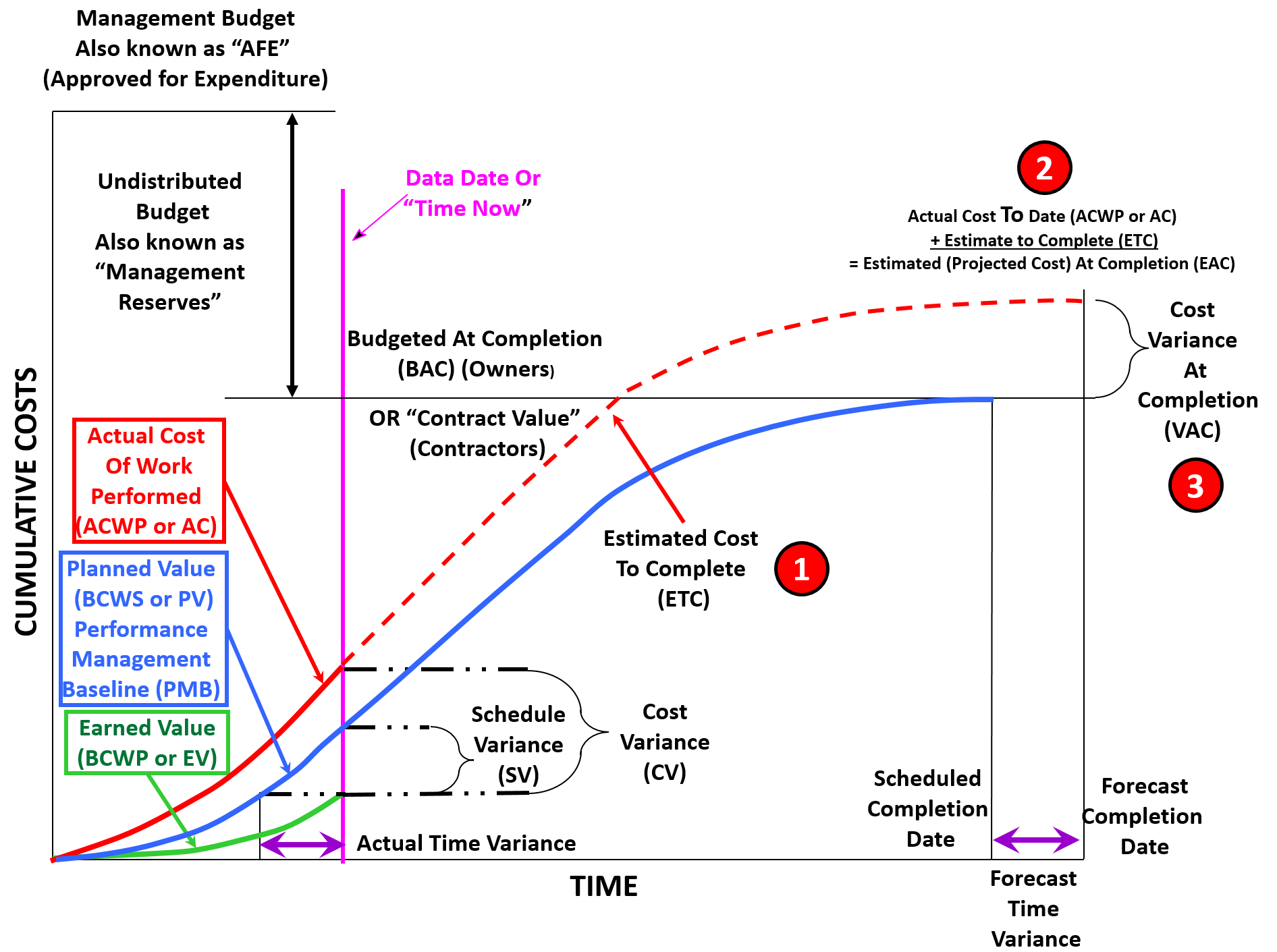
Figure 15 - Showing the Focus of this Section

Source: Adapted from DAU Gold Card KPI’s (2015)

While in the previous section our focus was on predicting the future completion date of the project, in this section, we are going to be focusing on the following:

• Estimated Cost to Complete, which is known as the Estimate To Complete (ETC) - This is an estimate of how much more money it will take to finish the remaining scope of work.

Estimate at Completion (EAC) which is calculated by taking the Actual Cost Of Work Performed (ACWP or AC) which are also known as “sunk costs” or “expended costs” and adding to that the Estimate to Complete which will give us the Estimate at Completion or EAC. In some industries, this is also known as the “Latest Projected Cost Estimate” or “LE” (Latest Estimate). There are 4 different formula’s which can be used and depending on the circumstances, can produce significantly different results. Which is why, unless we can clearly identify and justify the use of one formula over another, the “safest” way is to use the outcomes and from them, pick a “best case” value, a “worst case” value and a “most likely” value then applying the PERT formula, (see calculate the Mean, the sigma or standard deviation and then ask the client, sponsors or key stakeholders what “P” or “comfort level” they want and calculate the predicted finish date using that approach. Keep in mind that the higher the variance the more risky the calculations so whenever there is a large variance it is advisable to pick a higher “P” or “confidence” level. (i.e. If the stakeholders picked P90 and the variance was large, then the wise project control professional would recommend they use P95 or P98)

• Variance at Completion (VAC) which is the difference between the original baseline budget (BAC or for Contractors, Contract Value) and what the projected costs are. The Variance at Completion (VAC) is also applied to time as well as costs.

Assuming that our accounting/finance system is able to provide real time cost information down to the activity level or that we have implemented a system similar to that shown in Module 09.3 - Capturing Progress & Updating the Schedule, to close the accounting gap, we should be able to generate a curve which looks something like the one above which contains: 

1. Early Date Budgeted Cost of Work Scheduled
2. Late Date Budgeted Cost of Work Scheduled
3. Budgeted Cost of Work Performed (Earned Value)
4. Actual Cost of Work Performed

• From these 4 pieces of information, we can finish up our forward looking analysis (Forecasts).

09.5.3.3.1 CPI vs. TCPIeac

As we know from above, the formula to calculate the CPI is BCWP/ACWP or EV/AC for our PMI readers. And we also know the following metrics apply to CPI:

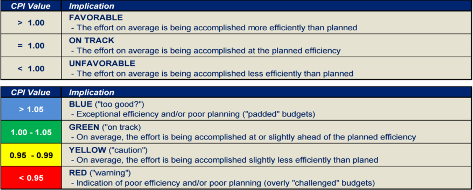
Figure 16 - CPI values from the NDIA’s Guide to Managing Programs Using Predictive Measures 

Source: Guide to Managing Programs Using Predictive Measures (2014) NDIA

• The TCIP(EAC) is the average future cost efficiency that must be maintained going forward in order to achieve a project’s EAC.

For a typical project, future efficiency will likely be similar to past efficiency. By comparing CPI and TCPI(eac), assessments can be made about the risk associated with achieving a project’s EAC.

• The formula to calculate TCIP(eac) = (BAC-BCWP)/(EAC-ACWP)

A second formula can also be used and that is Budgeted Cost of Work Remaining (BCWR)/Estimate to Complete (ETC)

A CPI of 0.91 indicates that, to date, $0.91 of work was done for every dollar spent on the project. Similarly, a TCPI(eac) of 1.11 indicates that $1.11 worth of work must be done for every dollar spent to meet the current EAC.

09.5.3.3.2 Independent Estimates at Completion’s (IEAC1 to IEAC4)

Given we have an ACWP and we are at the 33% elapsed time of the project, there are 5 formulas we can apply to the ACWP to predict or forecast the future cost, which is known as the Estimated Cost At Completion or more simply, “Estimate at Completion” or “EAC”. This also goes by other names i.e. in the telecommunications sector, this is known as the “Latest Estimate” or “LE”. Regardless of the name given to it, what we are trying to explain to our stakeholders as realistically as possible, what we believe the project is going to cost when it is completed.

All 5 formula start with the ACWP as that is a “sunk cost”- it has already been spent and has or should have no bearing on the future decisions and to that, we add the Estimated Cost to Complete (ETC). The ACWP + ETC = EAC; There are 5 formulas which can be used, 4 of them published by the NDIA and a 5th one added based on the collective experience of the GPC authors of this document:

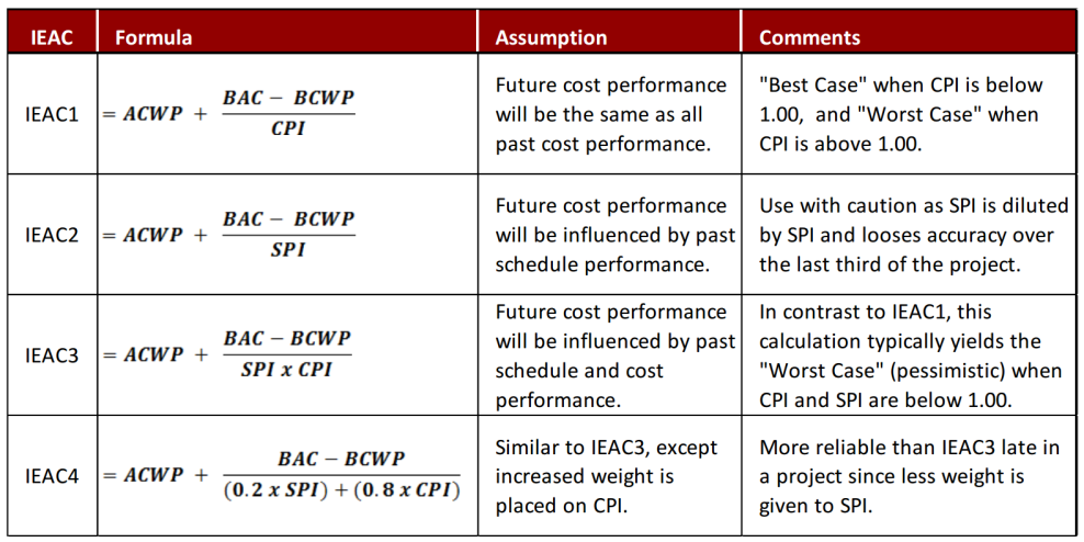
Figure 17 - 4 NDIA formulas to calculate Independent Estimate at Completion (IEAC)

Source: Guide to Managing Programs Using Predictive Measures (2014) NDIA pages 49-51

09.5.3.3.3 IEAC1 Example

Below is a real case study where the CPI was “so good to be true” actually happened and what actions the project manager took to “fix” the problem of too much budget.

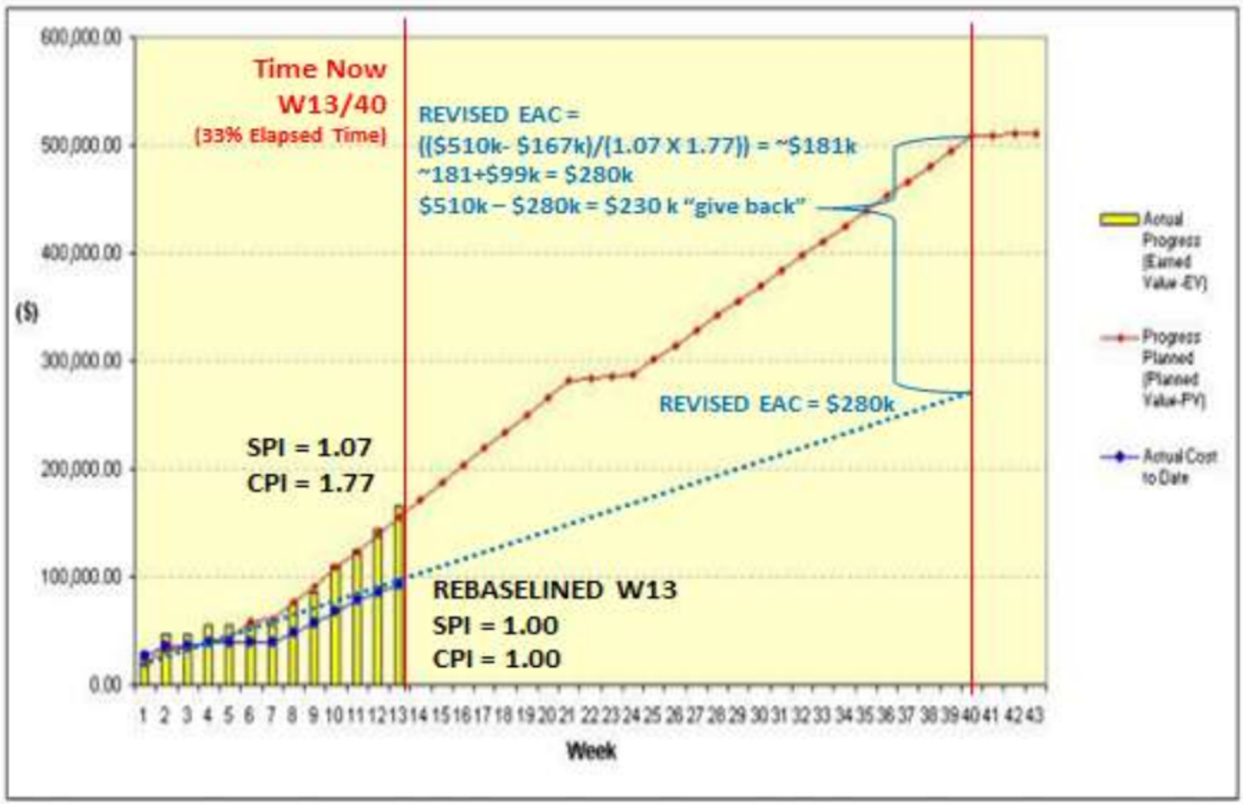
Figure 18 - Case Study Showing how to use SPI and CPI

Source: Dangdua, Danny as published by Giammalvo, Paul D (2013) "Practical Look at How Private Sector Entrepreneurial Contractors use Earned Value" PM World Journal Vol. II, Issue VII – July 2013

As we can see in the case study, while this project manager was 7% ahead of schedule (SPI 1.07) he was 77% UNDER budget (CPI 1.77).

What he did was to “give back” $230,000 allocated budget for use on other projects rather than keeping it tied up. For his professionalism in turning back allocated budget which was not necessary, he was awarded a letter of commendation from his Vice President.

• This is consistent with the concept that we only have 15% to 33% elapsed time “window of opportunity” to identify if our projects are in trouble, what is or are the root causes and what corrective action do we need to take to correct the problem. Failure to act in within this window of opportunity means our probability of being able to recover is very low if possible at all.

Because the only formula which takes into account the practice of “blowing the budget” in order to decrease the duration (crashing) which is what many owner organizations are willing to accept, the recommended “best tested and proven” practice for private sector contractors is to use IEAC3 = ACWP + (BAC-BCWP)/(SPI X CPI).

Once again, as professional practitioners, your expert judgement will be required to determine which formula is most appropriate given the specific situation you are in, but in general, private sector owners and contractors tend to favour IEAC3 as their “default” formula.

09.5.3.3.4 IEAC2 Example- Total Float vs SPI Analysis

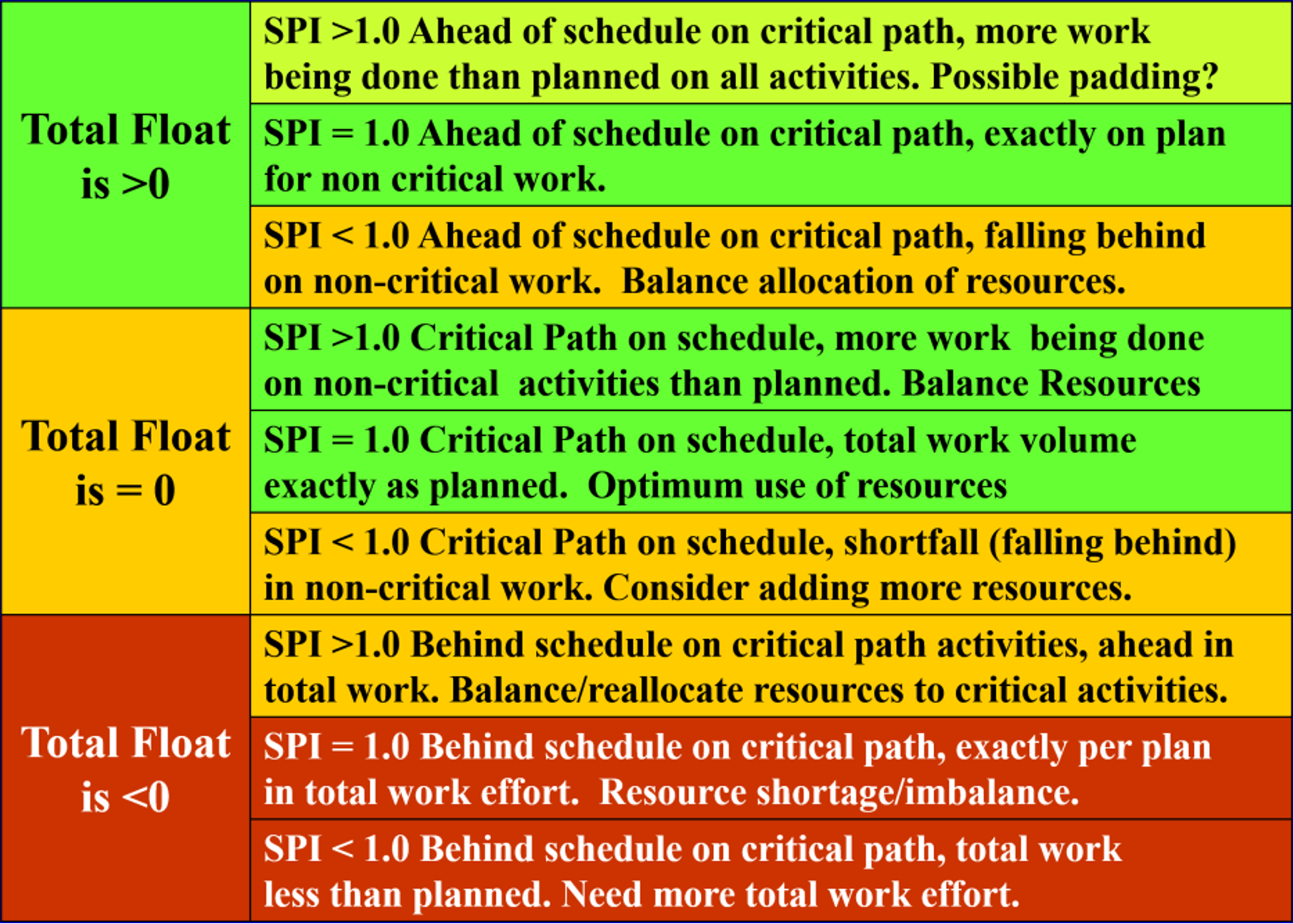
Figure 19 - Total Float vs SPI Analysis

Source: Adapted from AACE Skills and Knowledge of Cost Engineering, 5th Edition, page 16.8 figure 16.9

While the previous metrics all provide us with a high level view of our project without really telling us much about how to fix the problems the gauges are showing, this is a very powerful and useful tool for the project control professional to use at the working level:

• Total Float is >0 and SPI is >1: In this scenario while it may seem to be a perfect situation, this may well be one of those “too good to be true” situations. It may be that the project manager has built in too much schedule contingency, which while it may make him or her look good, does not necessarily mean that the project is being managed well. The project controller needs to review the contingency to see if in fact it is excessive.
• Total Float is >0 and SPI is = 1: In this scenario, we have positive float on the critical path (with a string of activities having > 1 total float) and with an SPI =1, we know we are exactly on schedule for all work. This project manager is not stressed out nor is he/she managing by crisis. He/she is deploying the available assets (human and equipment resources) to the best possible advantage by focusing on the critical path and building in a buffer or contingency on the critical activities, but without sacrificing work overall.
• Total Float is >0 and SPI is <1: This is an “early warning sign” or “risk trigger” that our project is headed for trouble. This is a common mistake of young or inexperienced project managers. They are right in focusing on the critical path but because they are falling behind in non-critical work, sooner or later they will find themselves with a new critical path. As a professional project controller, our advice to them is to focus on the near critical activities and add resources if possible to those activities as well as those on the critical path.
• Total Float is =0 and SPI is >1: In this scenario, we have a single critical path consisting of a string of activities with 0 Total Float. (Review Module 2.7- Managing Planning and Scheduling to learn how to calculate Total Float) But with an SPI > 1 it means we are ahead of schedule in overall work effort. While this is great, perhaps the project manager could reallocate some of the available resources off non-critical activities to the critical path and in doing so, shorten the schedule by a bit?
• Total Float is =0 and SPI is = 1: This is the project manager who will get the “Project Manager of the Month” award. He/she has a plan and is working that plan exactly. This is scenario is an indication the available resources are being deployed exactly as they should be, with the critical path taking priority, followed by the near critical activities and finally the non-critical activities last priority.
• Total Float is =0 and SPI is <1: This is another early warning sign or “risk trigger” that our project is either understaffed or that we have the wrong mix of resources working on the project and is headed for problems. As professional project controllers, we need to advise our project manager that he/she needs to be looking at the near-critical path activities and start to either reallocated available resources from non-critical to near critical activities and if that doesn’t work, then we need to add more resources to those near critical activities.
• Total Float is <0 and SPI is >1: This scenario is what happens if we ignore the first early warning signs or risk triggers. Our overall work effort is greater than planned, but because we have a new critical path and have ignored it, we now have negative float on one or more activities. Our advice to the project manager is to quickly reallocate resources from non-critical activities to the critical path and if that is not possible, then he/she needs to add more resources to work on the new critical path. This should never have happened if the advice of the project control professional was followed in Scenario 3 or 6 above.
• Total Float is <0 and SPI is = 1: As negative float should never happen, this is the end result if we fail to recognize the early warning signs in Scenario 6 above. Yes, our total overall work effort is fine (SPI = 1) but we either do not have the right resources or if we do have them they are working on non or less critical activities at the expense of the critical path.
• Total Float is <0 and SPI is <1: This is a total disaster and should never be allowed to happen. Here we have negative float and total work effort less than planned. Had we paid attention to the previous early warning signs or risk triggers in Scenarios 3, 6 and 7, and taken appropriate action by reallocating or adding more resources, we would not be in this situation.

09.5.3.3.5 IEAC5-Detailed Estimate To Complete

There is a 5th formula which the NDIA didn’t include which is commonly used when the actual costs or productivity either is not known or is subject to variability and needs to be validated for any specific application or context to provide future forecasts or predicted outcomes in terms of either time or cost.

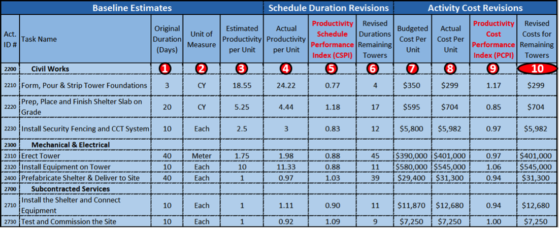
Figure 20 - Illustrating Using Productivity Modified SPI (PSPI) and PCPI to Revise Duration and Cost Forecasts

Source: Giammalvo, Paul D (2015) Course Materials Contributed Under Creative Commons License BY v 4.0

The above example is taken from a real project installing 75 cellular communications sites. A frag-net was created containing 8 Activities and as all sites were identical except for the physical location, P85 (mean plus 1 sigma) were used for cost and resource loading the schedules and as the basis to calculate durations and costs.

Because the contract was based on a unit price and because the scope was not well defined, the contract type was a “Job Order Contract” (JOC) which means when the 75 towers were inspected, the project was done and although there was a targeted time frame, because the scope was unknown it was not contractually mandated to finish on or before, although it was a desirable outcome.

To explain how to set up and use this table:

1. The original duration in days. For Activity 2210, Form Pour and Strip Tower Foundations it was 3 days long and required 55 cubic yards of concrete, which was not shown here but if you divide 55.65 CY of concrete by 3 days you come up with a baseline productivity of 18.55 CY per day.
2. Unit of Measure is self-explanatory
3. Productivity Per Unit in Place. As noted above, the productivity was 18.55 cubic yards per day. As this was an experienced crew who had been constructing these same sites for several years, we did NOT apply learning curve adjustments.
4. This was the actual productivity on the first unit, which was deemed to be “typical” of what could be expected in this area of operations.
5. Productivity Based Schedule Performance Index (PSPI)- By dividing the ESTIMATED productivity (3)/ACTUAL productivity (4) gave us the PSPI, (5) which in the example above is 0.77.
6. Revised Durations for Towers 2-75- taking the original duration (1) and dividing it by the SPI (5) gives us the REVISED DURATION. (3 days/0.77 = = 3.9 rounded to 4 days.
7. Budgeted Cost Per Unit- here we followed exactly the same process that we used for time, but this time using money instead. The original budgeted cost (BCWS or PV) for the Concrete in Place was $350/cubic yard.
8. Our actual costs in place (ACWP or AC) was $299/cubic yard.
9. Productivity Based Cost Performance Index (PCPI)- Dividing the Budgeted Costs Per Unit (8) of $350 by the Actual Unit Costs (9) of $299 we get a PCPI of 1.17.
10.  Predictive Future Unit Costs- Dividing $350 by 1.17 we get a predicted unit cost of $299. Because this was the first of 75 towers the CPI will be the same. But as we progress, we will continue to update the unit prices and use the past history to predict the future costs and durations as well.

This 5th formula not shown in the NDIA document is we use the SPI and CPI as we have shown in the above example OR we can look at the actual unit costs to date on the project and using those actual values, we look at the work remaining and using the actual costs to date, along with the actual productivity and using those values, ADJUST the remaining time or cost budgets either up or down to reflect as realistically as possible what the “real” or “true” cost of the project is going to be.

While this is the most accurate method, it is time consuming and tough to do unless the project has been shut down for one reason or another, as we have to mark up the drawings to show what work has been done and what work remains to be completed, then apply the cost adjustments ONLY to the remaining work. 

09.5.3.4 DASHBOARD REPORTS

While the previous graphics were created for illustration and learning purposes, it is important to recognize that what you often find  in real life projects are not perfect "S" Curves we see in textbooks and other reference documents.  To help provide a more realistic look at what dashboards actually look like, below are several examples taken from real life projects:   

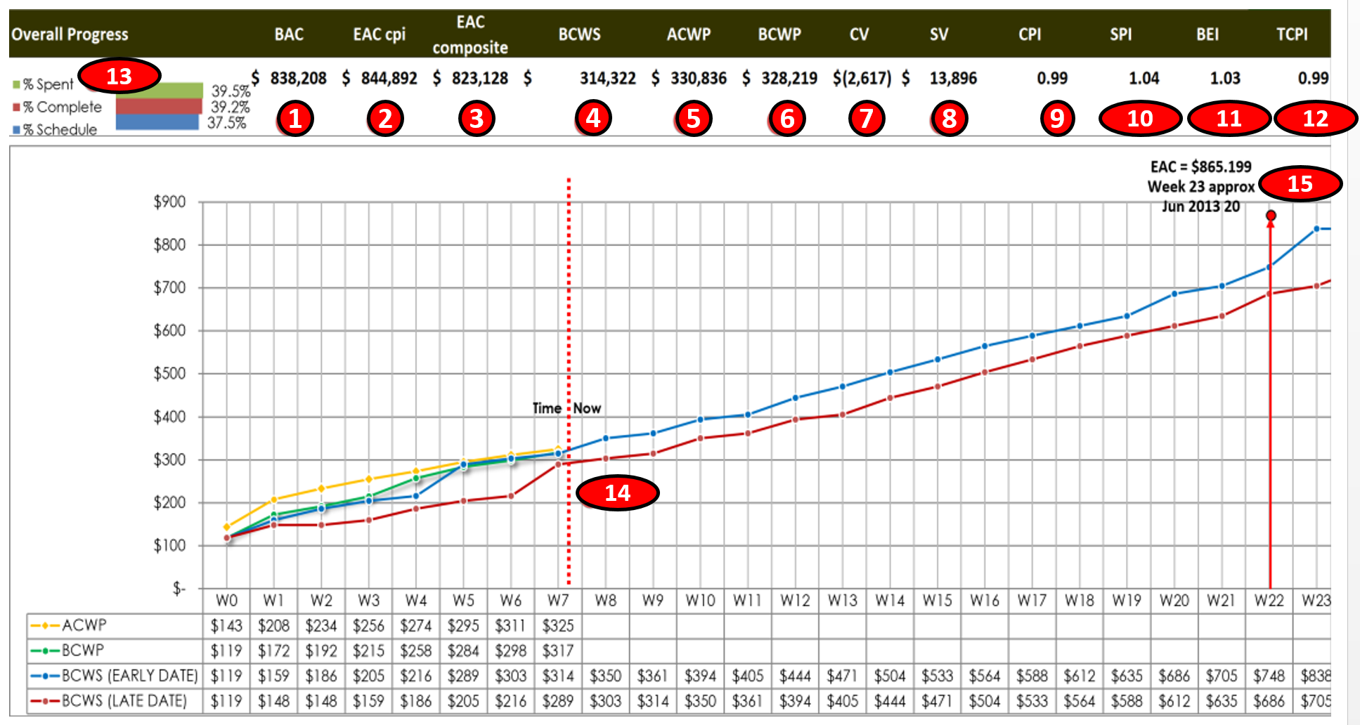
Figure 21 - S-Curve from a Real Progamme

Source: Giammalvo, Paul D (2015) Course Materials Contributed Under Creative Commons License BY v 4.0

In the example above, there are 7 projects in this program and this is the Level 1 Summary Report issued to management showing the overall program status as of the end of Week 7 of a 26 week program.  The chart explained:

1. The Budget At Completion for this program was $833,208
2. The Estimate At Completion using the CPI formula was $844,128
3. The Estimate At Completion using the CPI X SPI formula was $823,128
4. Cumulative BCWS to date was $314,322
5. Cumulative ACWP to date was $330,826
6. Cumulative BCWP to date was $328,219
7. Cost Variance (CV) was ($2,617) meaning we were $2,617 OVER budget
8. Schedule Variance (SV) was $13,896, meaning we are $13,896 AHEAD of schedule in terms of money
9. Cost Performance Index (SPI) is 0.99 meaning we are only 1% worth of work behind schedule
10. Schedule Performance Index (SPI) is 1.04, meaning we are 4% AHEAD of schedule in terms of work completed.
11. Baseline Execution Index (BEI) shows we have FINISHED 3% more activities than we had planned to finish by this date.
12. To Complete Performance Index (TCPI) means we only have to work at 99% efficiency for the remaining time to finish on time and within budget
13. We have spent 39.5% of our money budget; we have earned are 39.2% of our budget and only 37.5% of the time allowed has elapsed.
14. As of the end of Week 7, the projected completion date of this program is Week 23 and the P90 Estimated Cost at Completion is $865,199

Below is the same program, but this time using the metrics and Key Performance Indicators shown on the DAU Gold Card published using a TABULAR report format. Exactly the same information as above but shown in a different format.

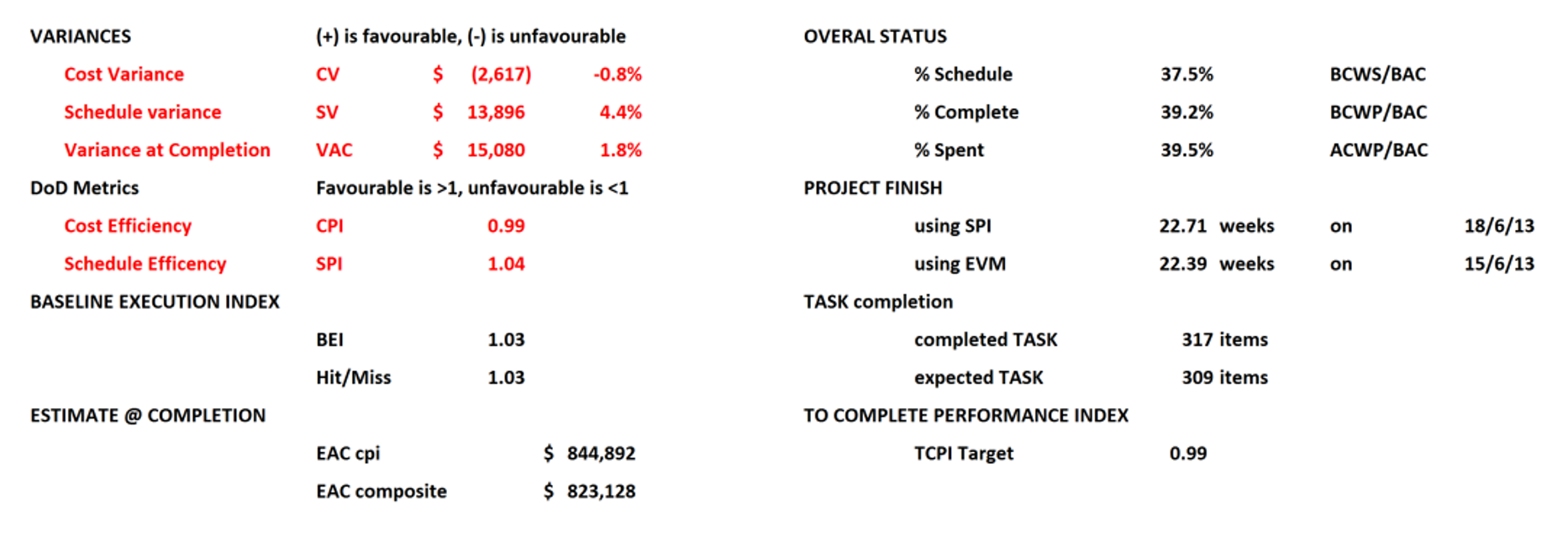
Figure 22 - Tabular Report Based on the DAU Gold Card KPI’s (2015)

Source: Giammalvo, Paul D (2015) Course Materials Contributed Under Creative Commons License BY v 4.0

Below is another example of a Web Based Project Status Dashboard:

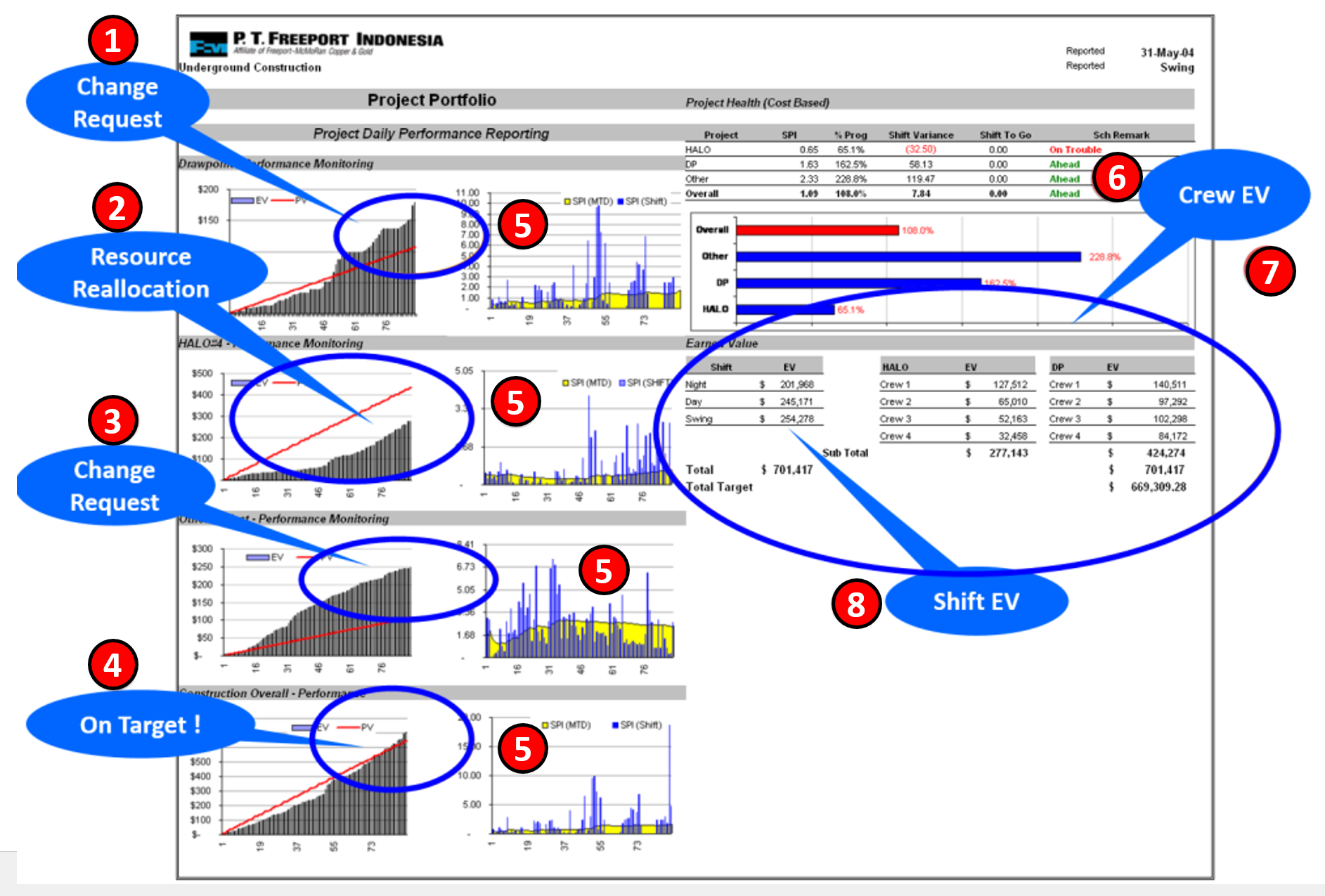
Figure 23 - Real Life Example of a Web Based Program Status Report Dashboard using Earned Value Metrics

Source: Wibiksana, Ridwan (2012) PM World Journal EVM Adapted for Underground Mining Operations Vol. I, Issue II – Sept 2012

To see the graphics more clearly, along with an explanation, this case study can be seen in more detail in this paper by Ridwan Wibiksana, CCP, PMP- “Earned Value Adapted for Use in Underground Mining”

The example above comes to us from a major mining giant. Because this was an OPERATIONAL project, instead of an S Curve, the client took the CAPEX budget and allocated it over a 365 day calendar. (3 shifts X 24 hours per day X 365 days per year). This resulted in a straight line which represents both the early and late date BCWS, and not the traditional “S” curve, but it served the same purpose, which was to compare the Earned Value (BCWP) vs the Planned Value (BCWS). Also worth noting is because this is a remote site mining camp, with a fixed pool of manpower and equipment, costs were not the driving force but how quickly ore could be extracted from the mine and processed to meet various contractual requirements, which is why the focus was on tracking and reporting SPI and not CPI. (The daily operating costs are the same regardless of whether the workforce is working efficiently or not, which is why the SPI was more important than the CPI, as that remains unchanged, the only exception being what materials are consumed:

1. In the first graph, we can see that management made a decision to change priorities, taking people from Project #2 and reallocating them to Project #1 and Project #3. The impacts of this change can be seen where the earned value (grey bars) go above the red line (BCWS) for Project #1.
2. We can see the impact of management’s decision to change priorities by pulling people off Project #2 and reallocating them to Projects #1 and #3. The impacts of this change can be seen where the earned value (grey bars) fall BELOW the red line (BCWS) for Project #2.
3. Again we can see the impact of management’s decision to change priorities by pulling people off Project #2 and reallocating them to Projects #1 and #3. The impacts of this change can be seen where the earned value (grey bars) are all ABOVE the red line (BCWS) for Project #3.
4. This is the PROGRAM level report, which shows that overall the three projects are right on track, with the grey bars showing the earned value slightly exceeding the red BCWS (planned value).
5. The blue bars indicate per SHIFT earned value and one of the challenges was to use Statistical Process Control charts (SPC) to determine why such big differences in per shift Earned Value and try to get the per shift performance (SPI) to be more consistent. That remains an on-going process today.
6. In this example, we can see that the HALO project (#2) is in trouble, but that was because of a conscious decision by management. However we can see that the other two projects plus overall are all ahead of schedule.
7. One of the very unique aspects of this case study is the client was using earned value at the crew level. This proved to be important as it enabled the superintendents to use the top performing crews as “schools”. What we would do is put some of the key people from the lower performing crews on the top performing crews for a week or so, as a means to show the lower performing crews how to work more efficiently and safely. We also used this as a means to recognize and reward those top performing teams for sustained performance in terms of both SPI and safety.
8. Lastly, as noted in 5, one of management’s concerns was the different productivity (measured by SPI) between the three shifts. So the crew earned value was rolled up and reported on a per shift basis, with the objective to try to narrow the differences between the day, swing and night shifts.

Another real life example has been provided to us by Rafael Davila in a posting on the Guild Forum, dated Tue, 2016-06-07 06:26:

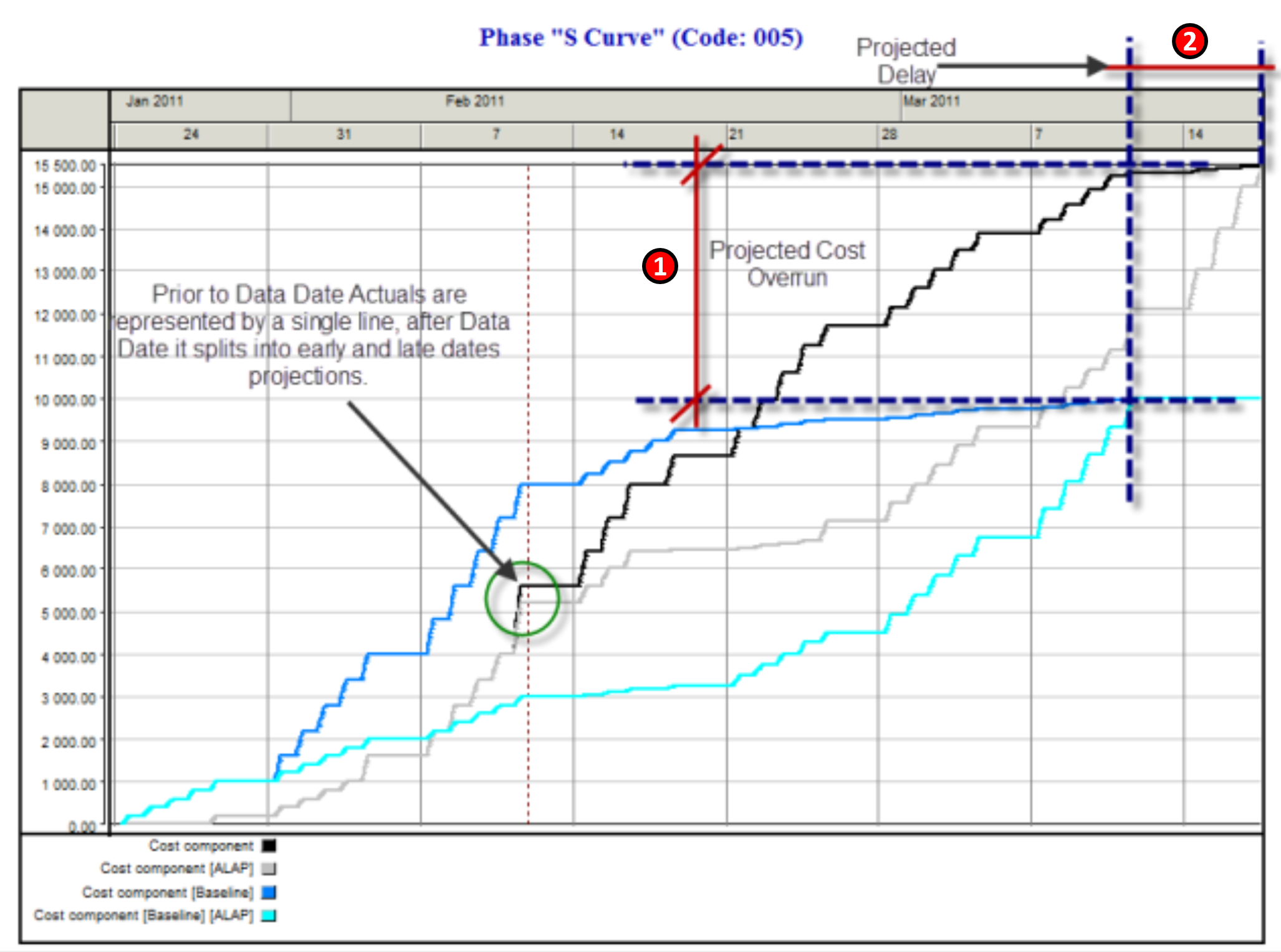
Figure 24 - Actual Example Showing the Projected Cost and Schedule Over-Runs

Source: Davila, Rafael Guild Forum, Tue, 2016-06-07 06:26 In this example, which was generated using Spider Software, we can clearly see (1) the difference between the original BCWS or PV and the Early and Late Date Projected Costs and (2) the Original Baseline Completion Date versus the Revised or Rebaselined Completion date.

Notice how “stair stepped” the lines are, which is a more realistic or accurate portrayal of money allocated over time, which in this case has been allocated on a daily basis. This is unlike many of the examples generated in Excel, MS Project or Primavera.  

09.5.3.5 THE PERIODIC PROGRESS REPORT

Worth revisiting and review prior to starting this next section is to determine who needs information, what information do they need, when to they need it and how do we get it to them.

To recap what we’ve covered in prior modules:

• Module 02-6 - Identifying And Engaging Stakeholders, we found out what information they needed, when do they need it and how do they want to receive it.
• Module 02-3 - Developing Individual Competencies, we found out what elements go into an effective communications model along with which medium is the most effective. This has important relevance for project control professionals for as we move towards a mobile based work environment, as well as the push to be more “environmental friendly” we are likely to see far less paper reports and many more web based reports, commonly referred to as “dashboards”. In the examples shown above, nearly all of them were “dashboard” (web based) reports rather than paper based.
• Module 3.2 - Validating Stakeholder Expectations, we were required to demonstrate that our stakeholder expectations were reasonable and that we could in fact meet them.
• Module 3.5 - Accepting Completed Deliverables, is where our stakeholders actually accepted work deliverables required.

The Periodic Progress Report, created by the contractor, for use by the contractor and by the owner will usually contain the following elements, but the project contract documents may often specify the required content:

1. A written review of progress of the contract made with reference to the activities detailed on the agreed Performance Measurement Baseline / Approved programme and detailing progress on each stage of the contract achieved during the reporting period i.e. design development, construction, manufacturing, installation and any relevant commissioning and testing. Progress should be measured up to and including the last day of the reporting period.
2. Details of any areas of concern or delay and any areas of technical difficulties incurred or expected should be specifically highlighted together with details of the contractor's actions and any necessary proposals for corrective action.
3. Hard copy of the agreed Performance Measurement Baseline / Approved programme detailing progress in bar chart format with comparisons of actual achievements and forecast performance with respect to the agreed baseline.
4. A turnaround document comprising a listing of ongoing, forthcoming (next 3 periods) and recently completed programme activities showing actual start and finish dates, percentage completion, forecast start and finish dates, remaining duration and a status in terms of +/- weeks.
5. Layout plans marked up to identify the extent of work completed in the reporting period and, cumulative to date for each major activity.
6. Comparative production curves and histograms showing actual versus planned performance in respect of major quantities.
7. Details of actual manpower on site for the period compared to that planned in the contractors baseline programme.

• Implicit in this is whether we are the Owner’s project control team or the Contractor’s we both have to know and understand not only the processes all of the tools and techniques above, as some of them provide the “big picture”, ideally suited for senior managers, while others are more appropriate for middle managers and of course, the majority of them are designed for the project control team to help advise and guide the project management team.

We also have to know and understand the outputs from all the processes, both from the perspective of the Owner as well as the Contractor.  

Figure 25 below outlines what can be a somewhat confusing relationship between Module 7 - Managing Project Planning and Scheduling and Module 9 - Managing Project Progress as it requires an initial and repeating set of processes between the Owner’s project control team and that of the Contractor’s project control team.

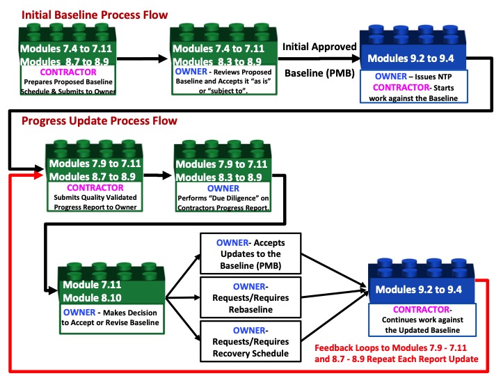
Figure 25 - Showing the High Level Relationship between Modules 7 and 9 from both the Contractor and Owner’s perspective

Source: Guild of Project Controls

STEP 1:

Upon awarding the contract, the contractor is normally required by the contract, to submit a detailed cost and resource loaded plan as a precondition to obtaining the Notice to Proceed (NTP) which shows how the contractor intends to execute the work within the time frames established in the contract. If the project is an internal project, then “Project Charter” (internal notice to proceed) is issued by the appropriate project sponsor authorizing work to commence against the approved plan.

To prepare the Initial Baseline the contractor follows the processes defined in Modules 7.1 through Module 7.10, and submits the relevant and appropriate deliverables to the Owner for acceptance as part of Module 7.11 processes.

STEP 2:

The owner reviews this baseline and either accepts it “as submitted” or “subject to” any reasonable changes the owner needs. After negotiations, an agreement is reached and the Owner then accepts the cost and resource loaded schedule containing all the relevant outputs from Modules 7.4-7.11 and it becomes the Project Performance Baseline (PMB).

At this point the Owner’s project control team also adds in any of their own cost and resource loaded activities to cover the Owner’s project overhead (e.g. Project Management, Safety, QA/QC) along with any owner supplied equipment or materials. The owner would also add in any contingency in terms of money or time.

This is what the starting PMB should typically looks like from both the OWNER and CONTRACTORS perspective, understanding that while the owner is able to see the contractors S Curve, it is highly unlikely the contractor will ever see the owners S Curve:

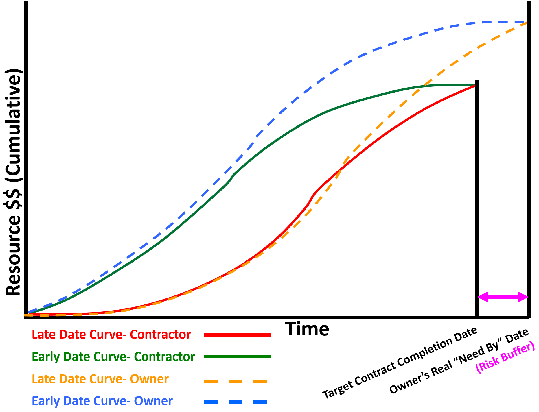
Figure 26 - Showing Owners Early and Late Date Curves vs Contractor’s Early and Late Date Curves

Source: Giammalvo, Paul D (2015) Course Materials Contributed Under Creative Commons License BY v 4.0

STEP 3:

The Owner issues the Notice to Proceed (NTP) or other authorization to the Contractor to commence work against the plan, which the contractor does, following the processes and producing the outputs defined in Modules 9.2, 9.3, 9.4 and 9.5 AND validated by the Contractor’s project control team by invoking the Quality Control processes identified in Modules 7.9 and 7.10, then submitting to the Owner through the processes defined in 7.11.

While there are contractual requirements in most standard contract documents, internal projects often do not have as strict reporting requirements, if for no other reason than for internal projects, the project manager is not being “paid” based on how much work he/she has completed. However the process remains the same whether the project is an internal or external one.

STEP 4:

At the end of the first and all subsequent reporting periods, the Contractor (External project) or Owner’s project manager (Internal project) submits a PROGRESS REPORT, which contains all the relevant analysis outputs defined in Modules 9.2, 9.3, 9.4 and 9.5 AND these outputs have been validated by running the quality control checks which were derived from Modules 7.9 and 7.10 and then submits the Periodic Progress Report to the owner by invoking the process defined in Module 7.11.

STEP 5:

When the Owner receives the Progress Report Update from the Contractor, the Owner’s project control team immediately follows the same quality control checklist from Modules 7.9, 7.10 and 7.11 that the Contractor followed but by looking at the outputs from the owner’s perspective, the owner can determine if the contractor is reporting what is legitimately happening against the plan or if the contractor is playing games with the schedule. (for more on this, see Pitaniello, S, Zack, J, Amadon, A and Federico, E. (2014) “Construction Scheduling Games Updated and Revisited”) 

STEP 6:  

Based on the outcomes of the “due diligence” done by the owner’s project control team, and their recommendations based on that analysis of the contractors periodic progress report, the Owner’s decision makers has 3 OPTIONS:

STEP 7: 

OPTION 1: ACCEPT THE PROGRESS UPDATE AS SUBMITTED by the contractor or internal project team, either “as submitted” or “subject to” implementing specific recommendations provided by the Owner’s Project Control Team.  If the schedule update is in substantial conformance to the baseline plan, with only minor differences in cost and time, and there are no changes to the logic or durations or if there were, they were explained and justified by the contractor and are acceptable to the owner, then the recommendation by the owner’s project control team to their project manager and other key stakeholders to “Accept the Update as Submitted”.

However in the event that OVERALL the schedule update is acceptable however there are minor changes which need to be made or small corrective actions, then the owner’s project control team would make the recommendation to their project manager or other key stakeholders to “ACCEPT the Progress Update SUBJECT TO" whatever action items the owner’s project control team recommends. These recommendations could take the form of recommending a change in the sequence of work, adding more critical resources or just about any other recommendations which do not impinge on the ability of the contractor to execute the work, provided it is done safely and within the constraints imposed by the contract. If this option is invoked, the project control team needs to check with your legal department to see whether these “recommendations” are in fact DIRECTIVES in which case, the contractor is most likely going to file a claim (e.g. for acceleration if the recommendation is to add more resources).

STEP 8:

OPTION 2: REJECT THE PROGRESS UPDATE AND REQUIRE A REBASELINE BE PREPARED, either by the Contractor or in some cases, by the Owner’s project control team, depending on the reason a Rebaseline is required.

In the event that the project as being built is “materially” or “significantly” different than what was originally planned, (and the “rule of thumb” is +/-10 variance is a “significant” variance) then we can recommend to the clients and key stakeholders that we REBASELINE the schedule. When Rebaselining, there are two options or approaches:

1. Leave the ACWP and BCWP to date UNCHANGED and only adjust the BCWS Early and BCWS Late Date Curves to reflect the changes. (+/-)
2. Zero Based Budgeting Method- In this method, we “close out” all the work completed to date and effectively create a new project baseline consisting of the work already done and the work remaining, and use the only known fact- ACWP to date as the starting point for the new project. 

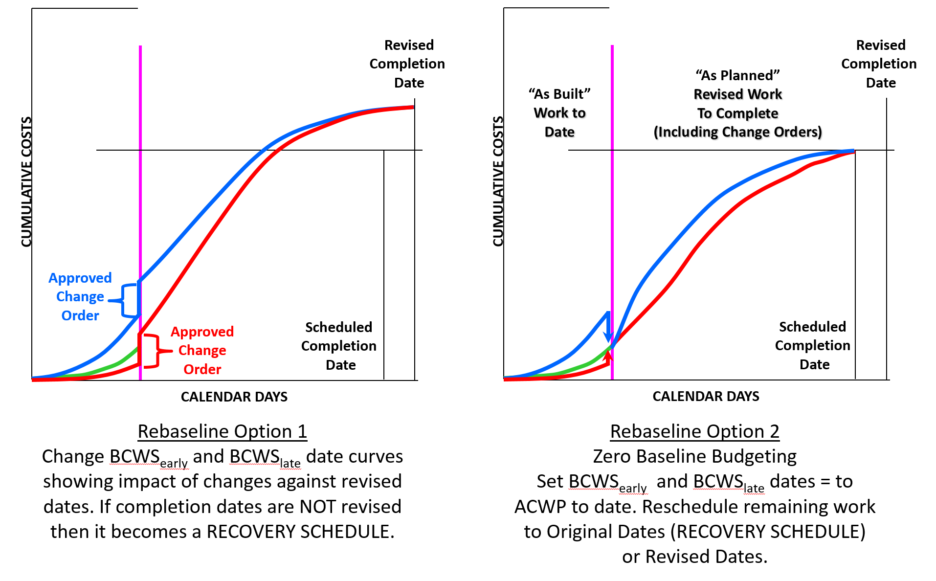
Figure 27 - Rebaseline and Recovery Schedules Illustrated 

Source: Giammalvo, Paul D (2015) Course Materials Contributed Under Creative Commons License BY v 4.0

STEP 9:

OPTION 3: REQUIRE (or REQUEST) that a “RECOVERY SCHEDULE" BE PREPARED, either by the Owner’s project control team (if the cause for a RECOVERY SCHEDULE to be necessary was primarily due to the OWNER’S errors/omissions (REQUESTED) or REQUIRED assuming the cause for a recovery schedule to be needed was largely the result of CONTRACTOR errors or omissions.

As we will see in Module 11 - Managing Change and Module 12 - Managing Forensic Analysis “recovery schedules” are often the cause of claims and dispute.

Applying this approach, the owner (project sponsor and key stakeholders) determine that the finish date (time) is of sufficient importance that it must be achieved at all costs. In this instance, the contractor is directed to accelerate the project by whatever combination of crashing, fast tracking and descoping if necessary is required to finish per the original deadline dates.

This acceleration is often the “root cause” reason for claims and disputes, as owner’s often claim it was the contractor who was responsible for the delays while the contractor often blames the owner for changes in scope that caused the delays. This topic will be covered in Module 11- Managing Change and Module 12 - Managing Forensic Analysis.

Regardless of which method is chosen, or who was at fault, normally, whenever a RECOVERY schedule is mandated, it will require that a REBASELINE schedule be created to show how the RECOVERY is going to be executed.  From a CONTRACTORS perspective, Option 1 is generally preferred as it enables the contractor to demonstrate the impact of the changes, while in most cases, owner’s prefer to see Option 2 as it gives them a more clear picture of what work is remaining and how it will be executed regardless of which dates have been agreed to.

STEP 10:

Based on the decisions by the Owner’s project control team, the Contractor continues to execute the project per the Updated Baseline.

Worth noting is that in the event the decision by the Owner has been to accelerate the contractor is still obligated to provide a “good faith” effort to work to the revised dates, although he/she may do so under protest, initiating whatever dispute resolution process is defined in the contract documents.

• This same 10 step process repeats each and every time an update is required, either on a regular schedule or an “ad hoc” request to address a specific problem, opportunity or issue.
• As we have to issue an update comparing current progress against the baseline schedule, we follow exactly the same procedure used to obtain the initial acceptance of our baseline.

09.5.4 OUTPUTS

• Current And Future (Predictive) Performance Metrics Calculated, Compared, Analyzed And Reported:
  • Critical Path Length Index (CCPLI)
  • Total Float Consumption Index (TFCI)
  • Earned Schedule (ES)
  • Time-Based Schedule Performance Index (Spit) Vs TSPied
  • Independent Estimated Completion Date – Earned Schedule (IECdes)
  • CPI Vs. TCPIeac
  • Independent Estimates At Completion’s (IEAC1 To IEAC5)
• Status Reports Produced, Analyzed And Published Proactive Corrective/ Preventive Actions 

09.5.5 REFERENCES & TEMPLATES

• GAO’s Best Practices in Capital Budgeting, Chapter 18 http://www.gao.gov/new.items/d093sp.pdf&nbsp;
• GAO’s Best Practices in Scheduling, Best Practice #9 pages 134-135 http://www.gao.gov/assets/600/591240.pdf
• GAO’s Best Practices in Capital Budgeting, Chapter 19, pages 270-271 http://www.gao.gov/new.items/d093sp.pdf
• GAO’s Best Practices in Scheduling, Best Practice #10 pages 150-151 http://www.gao.gov/assets/600/591240.pdf
• Guide to Managing Programs Using Predictive Measures (2014) NDIA http://www.ndia.org/Divisions/Divisions/IPMD/Documents/WorkingGroups/Pr…
• Pitaniello, S, Zack, J, Amadon, A and Federico, E. (2014) “Construction Scheduling Games Updated and Revisited” http://www.navigant.com/insights/library/construction/construction-foru…

Revisions & Change Control:

• Rev 1.01 - 1.04: Minor typographic and grammar amendments.
• Rev 1.05 - Amendments to "09.5.3.3.5 IEAC5-Detailed Estimate To Complete" and Figure 20 to better explain and differentiate between SPI and Productivity SPI coming from Columns 5 and 9 from Figure 20.

GPCCAR M09-5, Revision 1.05