Primavera P6 export to Excel. How to color WBS level automatically

After export activity table from Primavera P6 to Excel, it’s very hard to distinguish WBS level.
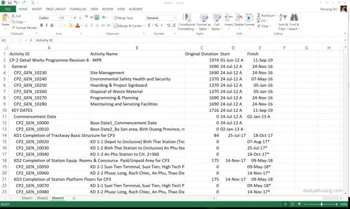
I will show you how to color WBS level automatically so we can have report like in P6.
- Step 1:
Follow this article to insert the "WBS Level" column : https://doduykhuong.com/2018/04/01/primavera-p6-export-to-excel-how-to-identify-wbs-level-for-activity/
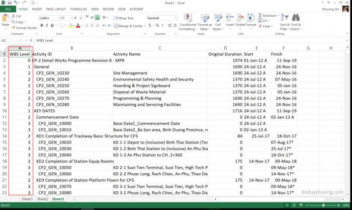
- Step 2:
Go to Conditional Formatting -> Manage Rules
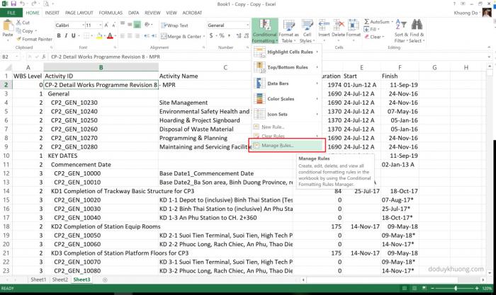
Create a New rule. Select Use a formula to determine which cells to format
In the formula box enter : =IF($A2=0,TRUE)
Select a color for WBS Level 0.

Click OK.
In the Applies to box, click the arrow icon to select the cells.
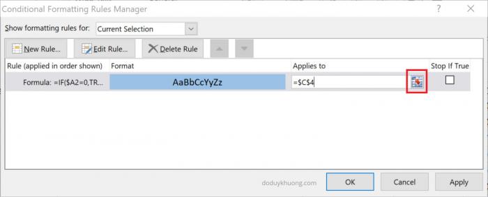
We select nearly the whole table.
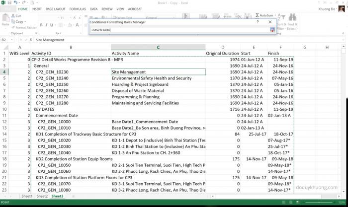
Click OK.
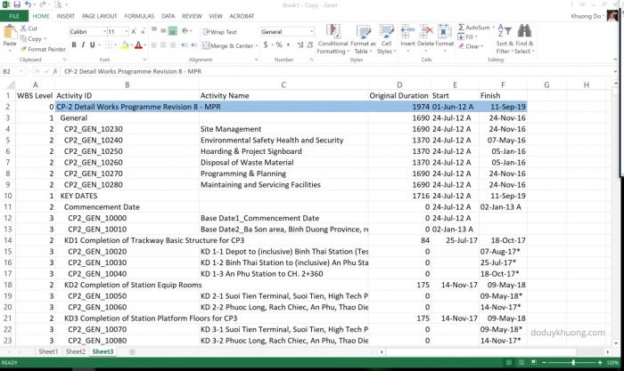
Now every WBS Level 0 will have green color.
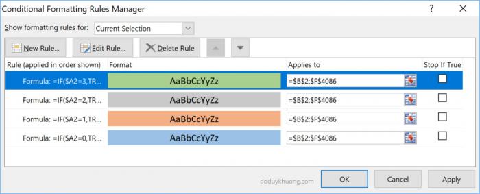
Then we create Rule for other WBS Level: 1, 2, 3
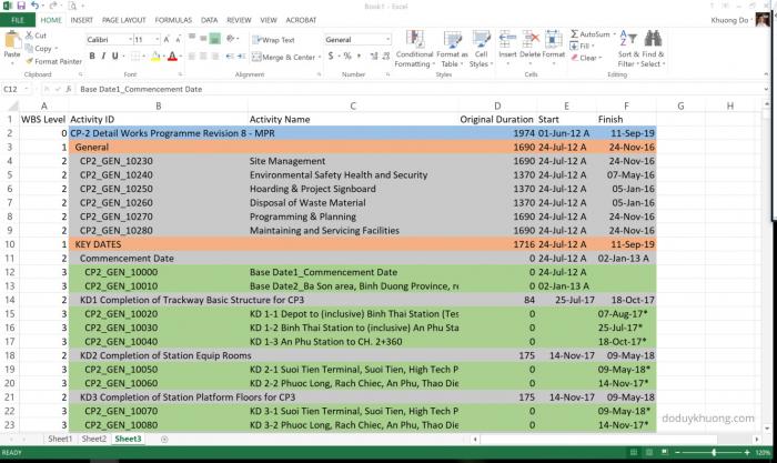
Now the report is very colorful :-)
About the Author : Khuong Do
Khuong Do is a Project Planner / Scheduler in Civil Engineering, Transportation, and Oil & Gas Industry. He has worked as a Primavera Consultant Specialist since 2006 and willing to share his passion for Primavera through lots of Tips & Trick on his personal blog : https://doduykhuong.com
 Printer-friendly version
- Login or register to post comments
 Send to friend


Comments
do not export it but copy
do not export it but copy data from p6 to excel
Help!when I export the file,
Help!
when I export the file, only activities & their details are shown (noWBS names are shown)
How do display the wbs names in the excel file?
I do mine a little
I do mine a little different
what you want to do is copy all the information from p6 to excel. Paste the data staring in column B. Then filter excel and filter where column C is blank, This will give you all of the WBS only rows. Then in column A2 add this formula which looks like this =LEN(B2)-LEN(TRIM(B2)). Copy this formula down in column A. This will give you the blank spaces before each character . This will reveal the indentation created by the P6 WBS. Next Filter Column A for each number then select all the row with that number and format those rows with a color. Filter column A for each value and give each different number row a different color. Now your excel sheet looks like P6 with the coloring.
No worries, I read your other
No worries, I read your other article ..... only after I figured out the formula..... :)
I also use an "isblank" statement in the conditional formatting to distinguish from WBS heading and activity, ie all activities have the same formatting similar to what is shown in P6. Only the "WBS Headings" are formatted.
=IF($A2=6,IF(ISBLANK($C2),TRUE))
Where "C" column is Activity ID
How do you input the WBS
How do you input the WBS values in the inserted column? manually?
?
?
Thanks Philip. I'm very happy
Thanks Philip. I'm very happy when you enjoy it :-)
Excellent post! Simplicity is
Excellent post! Simplicity is Beauty now, as is so often the case.
I presently run a macro to colour the row by WBS level, which means sometimes one needs to 'refresh' the colouring up. This method requires no VBA, and will apply as soon as the project calculates upon a change to any of the numbers in Column 'A'.
Really elegant solution!